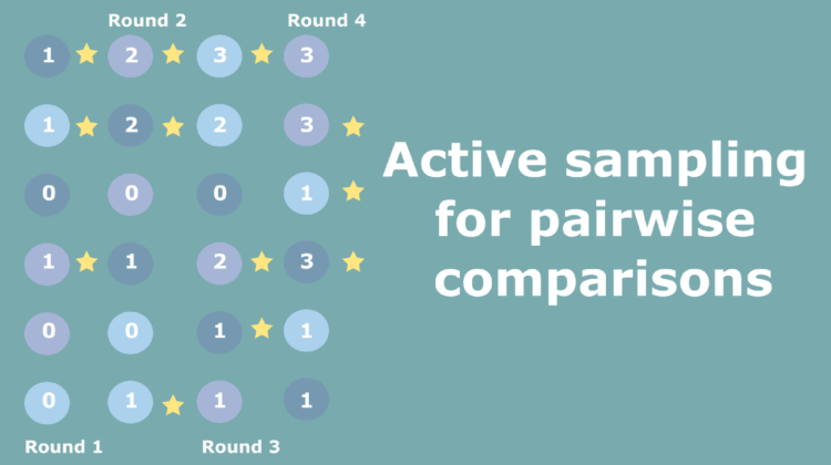
Lovers of chess, tennis or any other game with two competitors often face this problem — how to pair the players so that the ranking of players is determined in as few games as possible?
Similar problems occur in many industries, such as hospitality, food services, education, where entities are to be put onto consumer preference/skill scale, while running as few assessments as possible.
Pairwise comparisons are a common choice for ranking and scale inference. However, one of the drawbacks of pairwise comparisons is a large number of possible pairings. So the natural question is — how can we minimise the number of comparisons while gaining as much information as possible about the relative position of the entities on a scale. For example in a tennis tournament pairing me with Federer would be less informative than pairing him with Djokovic, as the outcome of our game would be obvious. As you might notice it is also important for player satisfaction from the game, as
This article is based on the paper “Active Sampling for pairwise comparisons via approximate message passing and information gain maximization” and comes along with the code, feel free to check it out! The method is called ASAP!
What has been done in the past?
Generally two types of methods are distinguished.
Sorting based: use a simple heuristic that similar in skill or in quality conditions should be paired. A well known example of such type of methods is Swiss Chess Tournament system, where in the first rounds chess players are paired at random, with every player participating in exactly the same number of games, and at later stages of the tournament players having comparable number of wins and looses are paired.
Information gain: Here results of pairwise comparisons are usually mapped to a one dimensional scale and pairs of conditions decreasing the uncertainty in the scale are formed. ASAP falls into that category!
Pipeline
Most active sampling methods for pairwise comparisons follow a similar pipeline.
Data: we start from the collected data so far, these would be outcomes of pairwise comparisons.
Scale: the data is then mapped to the scale. Information gain based methods assume a model of the scale, such as skills of the players being normally distributed, as in the famous TrueSkill algorithm (Thurstone Case V assumption), sorting based methods use a proxy to the scale, such as ranking of the conditions. Most information gain methods focus on approximate inference of the scale to improve the computational efficiency. ASAP does not use an approximate inference and greatly improves the accuracy of inferred scores.
Pair selection: Once the scale is available it is used for the selection of the next comparison to perform. Unlike other methods we focus on computational savings in that part of the algorithm.
Experiment: The next pairing of the conditions is selected and fed to the experiment, it can be a chess game or a questionary.
Data update: After we get the outcome, the data is updated.
Scale inference
For scale inference ASAP uses TrueSkill algorithm. For an intuitive and detailed explanation of the algorithm check out this article. We are interested in the normally distributed score variable, given the outcomes of the pairwise comparisons collected so far. Posterior distribution of the score variables provides us with the estimation of the mean of the score variable, as well as standard deviation (confidence/standard error) of the score variable.
TrueSkill uses sum-product algorithm with expectation propagation via moment matching. The algorithm is iterative with an overall complexity for the score inference k*O(n+t) where n is the number of conditions and t is the number of comparisons collected so far and k is the number of iterations to perform. More iterations result in better results, however, for growing number of comparisons t and compared conditions n can be prohibitively expensive for real-time applications. For that reason most methods approximate the posterior.
Expected information gain
Once the scale is available we can select the next comparison to perform that would improve the accuracy of the scale the most.
Stage 1: We start from the pairs collected so far. In the pairwise comparison matrix (square with number in the image above) every entry is the number of times condition in the corresponding row was selected over the condition in the corresponding column. Consider for example conditions two and three— two won three 3 times, three won two 1 time.
Stage 2: Now we simulate all possible comparison outcomes for every pair of conditions. Let’s look at the conditions two and three once again. We simulate the outcome in which two won on the top and three won at the bottom.
Stage 3: We then infer the scales for every possible simulated outcome
Stage 4: This is followed by the comparison of the new score distribution with the original scale with KL divergence. To obtain the expected information gain from the pairing we compute the expectation with respect to the probability of the outcome.
This procedure is repeated for all possible combinations of conditions, and, as you can imagine can be very computationally expensive.
Saving computations
Computing expected information gain for all possible pairings is expensive and we improve the speed in two ways:
- We only calculate expected information gain for a subset of the pairs
- Select comparisons in batches based on the minimum spanning tree
Selected EIG Evaluations
