For the previous post, please visit:
Introduction
After the success of LeNet in handwritten digit recognition, computer vision applications using deep learning came to a halt. Instead of feature extraction methods by filter convolutions, researchers preferred more handcrafted image processing tasks such as wavelets, Gabor filters, and many more. There were several reasons why the community did not push CNNs for many years to overtake more complex tasks. First of all, LeNet was good for MNIST but very few people believed that it is capable of dealing with more challenging data. After a while, it was not very interesting to work with MNIST over and over again. This links us to the second reason which was the lack of annotated data. Training neural networks requires an abundance of data and the need for more data increases as the model complexity (model size) increases. Since it is expensive to annotate data and CNNs were not really popular large-scale datasets were not available at the time. Last but not least, in order to train big models (assuming enough training data is provided) is a computationally expensive task. Each added layer of a deep learning model increases the number of parameters to be trained which significantly slows down the training. The hardware used in the ’90s took huge amounts of time to train even basic models and it was not feasible to design larger models.
All those reasons prevented new breakthroughs in the deep learning community for a long time. However, the last decade witnessed many exciting new projects and it feels like we are just getting started. In 2009, the ImageNet dataset is released with the title of ImageNet: A large-scale hierarchical image database[2]. Initially having 3.2 million annotated images, ImageNet now has more than 14 million images that are labeled in more than 20 thousand categories. That much of data encouraged many groups worldwide and excited them for the ImageNet Large Scale Visual Recognition Challenge (ILSRVC) which took place between 2010 and 2017. On the other hand, improvements were accelerated in hardwire with the millennium. NVIDIA released the first commercial GPU GeForce 256 in 1999 and GPU technology first used for deep learning in 2006 by Kumar Chellapilla et al[3]. Later on in 2009, Raina et al.[4] took a one step further for the popularity of GPUs on deep learning.
However, most of the credit goes to AlexNet in terms of the prevalence of GPU supported computation in deep learning literature. Winning the ILSRVC in 2012 by a quite large margin compared to the previous year’s winner, AlexNet proved that from now on, it is a necessity to employ state-of-the-art hardware for training the state-of-the-art models for the most complex task. AlexNet had more layers than LeNet has which brings a greater learning capacity. It is originally trained on the ImageNet dataset.
AlexNet with Tensorflow
This tutorial is intended for beginners to demonstrate a basic TensorFlow implementation of AlexNet on the MNIST dataset. For more information on CNNs and TensorFlow, you can visit the previous post at the beginning of this article. The reason for the usage of MNIST instead of ImageNet is simplicity, but the model can be used for any dataset with very few variations in the code.
First, needed libraries are imported.
import tensorflow as tf
import matplotlib.pyplot as pltfrom tensorflow.keras import datasets, layers, models, losses
The Data
Then, the data is loaded as in the LeNet implementation. One important notice is that the AlexNet model receives images with the size 224 x 224 x 3 however, MNIST images are 28 x 28. The third axis is expanded and repeated 3 times to make image sizes 28 x 28 x 3. It will be then resized at the first layer of the model to 224 x 224 x 3.
x_train,y_train),(x_test,y_test) = datasets.mnist.load_data()x_train = tf.pad(x_train, [[0, 0], [2,2], [2,2]])/255
x_test = tf.pad(x_test, [[0, 0], [2,2], [2,2]])/255x_train = tf.expand_dims(x_train, axis=3, name=None)
x_test = tf.expand_dims(x_test, axis=3, name=None)x_train = tf.repeat(x_train, 3, axis=3)
x_test = tf.repeat(x_test, 3, axis=3)x_val = x_train[-2000:,:,:,:]
y_val = y_train[-2000:]
x_train = x_train[:-2000,:,:,:]
y_train = y_train[:-2000]
The Model
AlexNet is one of the first examples of deep convolutional neural networks and it swept the competitions thanks to its high complexity (at the time) and the training procedure that is performed on GPUs. However, it was still not easy to train large networks due to vanishing gradient problems and long training times. AlexNet is large enough to learn the patterns in the ImageNet dataset but very shallow compared to today’s models. Why AlexNet could not be designed deeper becomes clearer after understanding the residual connections in ResNet.
The first layer (resizing layer) of the model does not exist in the original implementation since the data were already compatible with the model in terms of image size. MNIST images were interpolated bilinearly such that the new sizes are 224 x 224 (also one more dimension for 3 channels).
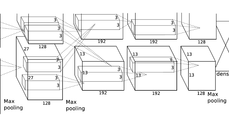
The first five layers are similar to LeNet layers in a sense. The layers consist of 96 filters with the size of 11 x 11, 256 layers with the size of 5 x 5, 384 layers with the size of 3 x 3, 384 layers with the size of 3 x 3, and finally 256 liters with the size of 3 x 3, respectively. Unlike LeNet, AlexNet uses ReLU[5] activation function. ReLU does not involve exponentiation, which is computationally expensive, thus ReLU is very cheap to calculate. It also reduces the effects of vanishing gradient and resembles the mechanism of biological cells. Yet, ReLU sometimes leads to dying neurons and it is advised to keep track of the activations during the first epochs of the training.
Another new concept is batch normalization, which is a common trick to make training go smooth and stable. In smaller networks, the data is normalized during preprocessing and fed into the models. Nevertheless, in larger models normalization procedure is repeated between layers by normalizing the layer activations with 0 mean and 1 variance. Reasonably, batch normalization is performed after convolution and before nonlinear activation and subsampling because the normalization is intended to be done on actual neuron activations.
The resulting tensor (1 x 1 x 256) is flattened and fed into fully connected layers. After passing two hidden layers having the sizes of 4096, final class scores (for 10 classes) are obtained by softmax operation. Here, dropout is a measure to prevent overfitting. In the model below, half of the neurons in hidden fully connected layers are shut down randomly. During each forward passing of the training samples, a specified fraction of the activations in a layer is set to 0, and in order to keep the mean activation level of the layer remaining activations are divided by dropout probability (in this case divided by 0.5 or simply multiplied by 2). During test time dropout is not performed.
model = models.Sequential()model.add(layers.experimental.preprocessing.Resizing(224, 224, interpolation="bilinear", input_shape=x_train.shape[1:]))model.add(layers.Conv2D(96, 11, strides=4, padding='same'))
model.add(layers.BatchNormalization())
model.add(layers.Activation('relu'))
model.add(layers.MaxPooling2D(3, strides=2))model.add(layers.Conv2D(256, 5, strides=4, padding='same'))
model.add(layers.BatchNormalization())
model.add(layers.Activation('relu'))
model.add(layers.MaxPooling2D(3, strides=2))model.add(layers.Conv2D(384, 3, strides=4, padding='same'))
model.add(layers.Activation('relu'))model.add(layers.Conv2D(384, 3, strides=4, padding='same'))
model.add(layers.Activation('relu'))model.add(layers.Conv2D(256, 3, strides=4, padding='same'))
model.add(layers.Activation('relu'))model.add(layers.Flatten())model.add(layers.Dense(4096, activation='relu'))
model.add(layers.Dropout(0.5))model.add(layers.Dense(4096, activation='relu'))
model.add(layers.Dropout(0.5))model.add(layers.Dense(10, activation='softmax'))model.summary()
The model summary is as follows:
Model: "sequential" _________________________________________________________________ Layer (type) Output Shape Param # ================================================================= resizing (Resizing) (None, 224, 224, 3) 0 _________________________________________________________________ conv2d (Conv2D) (None, 56, 56, 96) 34944 _________________________________________________________________ batch_normalization (BatchNo (None, 56, 56, 96) 384 _________________________________________________________________ activation (Activation) (None, 56, 56, 96) 0 _________________________________________________________________ max_pooling2d (MaxPooling2D) (None, 27, 27, 96) 0 _________________________________________________________________ conv2d_1 (Conv2D) (None, 7, 7, 256) 614656 _________________________________________________________________ batch_normalization_1 (Batch (None, 7, 7, 256) 1024 _________________________________________________________________ activation_1 (Activation) (None, 7, 7, 256) 0 _________________________________________________________________ max_pooling2d_1 (MaxPooling2 (None, 3, 3, 256) 0 _________________________________________________________________ conv2d_2 (Conv2D) (None, 1, 1, 384) 885120 _________________________________________________________________ activation_2 (Activation) (None, 1, 1, 384) 0 _________________________________________________________________ conv2d_3 (Conv2D) (None, 1, 1, 384) 1327488 _________________________________________________________________ activation_3 (Activation) (None, 1, 1, 384) 0 _________________________________________________________________ conv2d_4 (Conv2D) (None, 1, 1, 256) 884992 _________________________________________________________________ activation_4 (Activation) (None, 1, 1, 256) 0 _________________________________________________________________ flatten (Flatten) (None, 256) 0 _________________________________________________________________ dense (Dense) (None, 4096) 1052672 _________________________________________________________________ dropout (Dropout) (None, 4096) 0 _________________________________________________________________ dense_1 (Dense) (None, 4096) 16781312 _________________________________________________________________ dropout_1 (Dropout) (None, 4096) 0 _________________________________________________________________ dense_2 (Dense) (None, 10) 40970 ================================================================= Total params: 21,623,562 Trainable params: 21,622,858 Non-trainable params: 704The model is compiled and trained as in the previous post where LeNet is implemented. The choice of the Adam optimizer and the mathematical background of the optimizers are the topics of another post. However, Adam is the most common choice among the deep learning community for adaptively updating the learning rate.
model.compile(optimizer='adam', loss=losses.sparse_categorical_crossentropy, metrics=['accuracy'])history = model.fit(x_train, y_train, batch_size=64, epochs=40, validation_data=(x_val, y_val))Epoch 1/40 907/907 [==============================] - 38s 34ms/step - loss: 0.7459 - accuracy: 0.7291 - val_loss: 0.1064 - val_accuracy: 0.9735
Epoch 2/40 907/907 [==============================] - 31s 34ms/step - loss: 0.1237 - accuracy: 0.9665 - val_loss: 0.0816 - val_accuracy: 0.9790
...
Epoch 40/40 907/907 [==============================] - 32s 36ms/step - loss: 0.0123 - accuracy: 0.9970 - val_loss: 0.0465 - val_accuracy: 0.9930
The accuracy rises up very quickly in the validation set and fluctuates above 98% throughout the training. Training loss decreases consistently as expected.
fig, axs = plt.subplots(2, 1, figsize=(15,15))axs[0].plot(history.history['loss'])
axs[0].plot(history.history['val_loss'])
axs[0].title.set_text('Training Loss vs Validation Loss')
axs[0].set_xlabel('Epochs')
axs[0].set_ylabel('Loss')
axs[0].legend(['Train', 'Val'])axs[1].plot(history.history['accuracy'])
axs[1].plot(history.history['val_accuracy'])
axs[1].title.set_text('Training Accuracy vs Validation Accuracy')
axs[1].set_xlabel('Epochs')
axs[1].set_ylabel('Accuracy')
axs[1].legend(['Train', 'Val'])
Test accuracy came out at 98.79%.
model.evaluate(x_test, y_test)313/313 [==============================] - 2s 7ms/step - loss: 0.0809 - accuracy: 0.9879
[0.08089840412139893, 0.9879000186920166]
alexnet_tensorflow.ipynb
Conclusion
AlexNet started a revolution in the computer vision community and paved the road for many other deep learning models. In the following years, ILSRVC became much more competitive and winner models reached higher and higher accuracies. The use of GPUs, ReLU activations, batch normalization layers, and dropout mechanism were all new compared to the predecessor model, LeNet. In this implementation, a relatively light MNIST dataset is used for fast training and simplicity, for which AlexNet is an overkill. The original model is trained and evaluated on ImageNet in 2012.
Hope you enjoyed it. See you in the following CNN models.
Best wishes…
mrgrhn
References
- Krizhevsky, Alex & Sutskever, Ilya & Hinton, Geoffrey. (2012). “ImageNet Classification with Deep Convolutional Neural Networks”. Neural Information Processing Systems. 25. 10.1145/3065386.
- Deng, Jia & Dong, Wei & Socher, Richard & Li, Li-Jia & Li, Kai & Li, Fei Fei. (2009). “ImageNet: a Large-Scale Hierarchical Image Database”. IEEE Conference on Computer Vision and Pattern Recognition. 248–255. 10.1109/CVPR.2009.5206848.
- Chellapilla, Kumar & Puri, Sidd & Simard, Patrice. (2006). “High Performance Convolutional Neural Networks for Document Processing”.
- Raina, Rajat & Madhavan, Anand & Ng, Andrew. (2009). “Large-scale deep unsupervised learning using graphics processors”. Proceedings of the 26th International Conference On Machine Learning, ICML 2009. 382. 110. 10.1145/1553374.1553486.
- Nair, Vinod & Hinton, Geoffrey. (2010). “Rectified Linear Units Improve Restricted Boltzmann Machines”. Proceedings of ICML. 27. 807–814.