Supervised learning algorithms classify with two categories: classification and regression. In regression based algorithms, the target variable consists of continuous values and we try to estimate these values. Classification based algorithms, on the other hand, consist of categorical data (such as yes-no). Of course, this classification target variable can also consist of multiple categorical data (good-medium-bad). Many of the classification-based algorithms use probability measures to categorize the best estimate. The Naive Bayes Classifier is one of these methods. Let’s examine how this classification is made.
When a meteorologist provides a weather forecast, precipitation is typically predicted using terms such as “70 percent chance of rain.” These forecasts are known as probability of precipitation reports. Have you ever considered how they are calculated? It is a puzzling question, because in reality, it will either rain or it will not.
These estimates are based on probabilistic methods, or methods concerned with describing uncertainty. They use data on past events to extrapolate future events. In the case of weather, the chance of rain describes the proportion of prior days with similar measurable atmospheric conditions in which precipitation occurred. A 70 percent chance of rain therefore implies that in 7 out of 10 past cases with similar weather patterns, precipitation occurred somewhere in the area.
Just as meteorologists forecast weather, naive Bayes uses data about prior events to estimate the probability of
future events. Let’s examine how this algorithm works with basic principles of probability:
The basic statistical ideas necessary to understand the naive Bayes algorithm have been around for centuries. The technique descended from the work of the 18th century mathematician Thomas Bayes, who developed foundational mathematical principles (now known as Bayesian methods) for describing the probability of events, and how probabilities should be revised in light of additional information.
We can say that the probability of an event is a number between 0 and 100 percent, which, given the available evidence, has the chance to occur. The lower the probability, the less likely the event will occur. The probability of 0 percent indicates that the event will never happen, 100 percent probability indicates that the event will never happen.
Classifiers based on Bayesian methods utilize training data to calculate an observed probability of each class based on feature values. When the classifier is used later on unlabeled data, it uses the observed probabilities to predict the most likely class for the new features. It’s a simple idea, but it results in a method that often has results on par
with more sophisticated algorithms.
Typically, Bayesian classifiers are best applied to problems in which the information from numerous attributes should be considered simultaneously in order to estimate the probability of an outcome. While many algorithms ignore features that have weak effects, Bayesian methods utilize all available evidence to subtly change the predictions. If a large number of features have relatively minor effects, taken together their combined impact could be quite large.
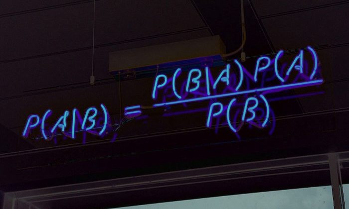
First, let’s explain Bayes’ theorem:
Bayes’ theorem is an important subject that is studied in probability theory. This theorem shows the relationship between conditional probabilities and marginal probabilities within a probability distribution for a random variable. In this way, Bayes’ theorem explains an acceptable relationship. The probability value for a conditional A event (ie, event A, although event B is known) to event B as an ‘event’ examined in the probability theory differs from the probability value for event B to event A (ie, event B where event A is known). However, there is a very specific relationship between these two opposite conditions, and this relationship is called the Bayes Theorem.
P(A|B): Probability of event A when event B is known
P(B|A): Probability of event B when event A is known
P(A): Probability of event A
P(B): Probability of event B
Now let’s continue with the example. For example; feature is the weather (x) and whether or not playing football is our class variable (y). Let’s try to predict whether or not to play football according to the weather with Naive Bayes algorithm. The training data is as follows:
Now let’s ask a question and calculate its probability:
For example, our question is: Do I play when the weather is rainy?
P(Yes|Rainy)=P(Rainy|Yes)*P(Yes)/P(Rainy)
First, let’s look at the possibility of being rainy when it is known to be yes: 3 out of 9 yes are rainy: P (Rainy | Yes) = 3/9 = 0.33 probability is obtained.
Let’s look at the possibilities of being “Yes” and “Rainy”:
Of the 14 observations in total, 9 are “Yes”. P (Yes) = 9/14 = 0.64
Of the 14 observations in total, 5 are “Rainy”. P (Rainy) = 5/14 = 0.35
Now let’s write down the values and calculate the probability of playing when the weather is rainy:
P(Yes|Rainy)=P(Rainy|Yes)*P(Yes)/P(Rainy)=0.33*0.64/0.35=0.60
In other words, when the weather is rainy, the probability of playing football was determined as 0.60. Of course it is a probability value calculated here. However, we expect a clear prediction, such as “I play” or “I don’t play”. The Naive Bayes algorithm rounds according to the high probability when making this estimate. Here comes the result of “I play with 60% probability”. According to the Naive Bayes algorithm, this situation is determined as “Yes”.
Of course, we made a guess here using a single column feature. If there were multiple features, we would do the same for each column. In other words, in Naive Bayes, each feature would be determined independently. When more than one feature is used, the formula is as follows:
- Since each feature is considered independent from each other, it can perform better than models such as logistic regression.
- It can do well with little data.
- It can be used with continuous and discrete data.
- It can work well in high dimensional data.
- Relationships between variables cannot be modeled since the features are assumed to be independent from each other.
- You may face zero probability problem. Zero probability is the situation that we want, for example, not to be present in the data set. The simplest method for this is to eliminate this possibility by adding a minimum value to all data (usually 1). This situation is also called estimation using Laplace.
Gaussian Naive Bayes: If our features consist of continuous data, we assume that this data comes from a Gaussian distribution, in other words, a normal distribution.
Multinomial Naive Bayes:As we said earlier, the Naive Bayes algorithm is used in multi-class categories (such as good-medium-bad).
Bernoulli Naive Bayes:Classes here consist only of binary values (such as good and bad).
So far, we have touched on the purpose of Naive Bayes algorithm, how it predicted, its advantages, disadvantages and types. Let’s apply an application using R programming language:
Before we start the application, let’s install the necessary packages and create libraries. The packages to be installed are as follows:
install.packages(“tidyverse”)
install.packages(“caret”)
install.packages(“mlbench”)
install.packages(“klaR”)
install.packages(“ggplot2”)
install.packages(“magrittr”)
install.packages(“lattice”)
install.packages(“e1071”)
install.packages(“datasets”)library(tidyverse)
library(caret)
library(mlbench)
library(klaR)
library(ggplot2)
library(magrittr)
library(lattice)
library(e1071)
library(datasets)
Let’s apply the Naive Bayes algorithm to the “PimaIndianDiabetes2” data set in the “mlbench” library and start our analysis.
First, let’s upload the data set to the system and look at its descriptive statistics:
data(“PimaIndiansDiabetes2”)
summary(PimaIndiansDiabetes2)
When we look at the descriptive statistics, we see that there are missing values. Let’s continue our analysis by removing these observations from the data set.
PimaIndiansDiabetes2<-na.omit(PimaIndiansDiabetes2)
Thus, we have removed lost observations from the dataset. Let’s look at the descriptive statistics again:
summary(PimaIndiansDiabetes2)
When we look at the output, we can say that there are 392 observations. Here, the diabetes variable is our target variable and includes test results for diabetes disease made to 392 people. Accordingly, the test of 262 people is negative, the test of 130 people is positive, and this variable is tried to be explained by 8 different features. Now let’s try to estimate the values in the diabetes variable using the Naive Bayes algorithm. First, let’s divide the data set into 2 different groups as training and test data. The R codes that should be written for this are shown below:
set.seed(123)
training.samples<-PimaIndiansDiabetes2$diabetes %>%
createDataPartition(p=0.8,list=FALSE)
train.data<-PimaIndiansDiabetes2[training.samples, ]
test.data<-PimaIndiansDiabetes2[-training.samples, ]
The important thing here is how to choose training data. We determine the training data randomly. The “set.seed” command is one of the functions required to generate random data in R, and we can achieve more successful modeling when the set.seed function is assigned with the value 123. 80% of our observations consist of education data and 20% consists of test data. Now, let’s train our model with the Naive Bayes algorithm using this training data:
model<-NaiveBayes(diabetes~.,data=train.data)
We applied the training data using the Naive Bayes function in R. Now let’s test it with our test data using this model and calculate our accuracy rate:
predictions<-model %>% predict(test.data)
mean(predictions$class==test.data$diabetes)
[1] 0.8205128
Thus, we can say that our success rate is 82%. Of course, we have trained our data here by using all of our features. Let’s remove some features and apply the Naive Bayes algorithm again.
In the previous article, we decided on which variables would be removed from the model by applying stepwise logistic regression with logistic regression analysis. You can reach the article I wrote about logistic regression analysis from the link below:
The features that remained in the model with stepwise logistic regression were pregnant, glucose, mass, pedigree and age. Let’s re-apply the Naive Bayes algorithm using these features. First, let’s create a new data set from these features. R codes are shown below:
data2<-data.frame(diabetes=PimaIndiansDiabetes2$diabetes,pregnant=PimaIndiansDiabetes2$pregnant,glucose=PimaIndiansDiabetes2$glucose,mass=PimaIndiansDiabetes2$mass,pedigree=PimaIndiansDiabetes2$pedigree,age=PimaIndiansDiabetes2$age)
Now, let’s separate this data set as retraining and testing data:
set.seed(123)
training.samples<-data2$diabetes %>%
createDataPartition(p=0.8,list=FALSE)
train.data<-data2[training.samples, ]
test.data<-data2[-training.samples, ]
Thus, 80% of the data set was reserved as training and 20% as test data. Let’s apply the Naive Bayes algorithm and look at the results:
model<-NaiveBayes(diabetes~.,data=train.data)
predictions<-model %>% predict(test.data)
We trained the training data with the Naive Bayes algorithm and predicted the test data. Now let’s look at the output:
We see that we received an error here. As we mentioned earlier, one of the disadvantages of the Naive Bayes algorithm was that it gave zero probability error. To deal with this, Laplace estimation needs to be applied. So we can get rid of this error by adding “1” to each observation. For this, there is a “naiveBayes” function in the package “e1071” in R Here, “laplace” parameter value can be specified as “1”. R codes are shown below:
model<-naiveBayes(diabetes~.,data=train.data,laplace = 1)
predictions<-model %>% predict(test.data)
mean(predictions==test.data$diabetes)
[1] 0.8076923
Yes, so our accuracy rate was calculated as 80%. When we analyzed using all the features in the data set, we said that it was 82%. According to the Naive Bayes algorithm, we have a higher accuracy rate when all features are used.
Of course, the Naive Bayes algorithm also works in multi-class categories. Let’s make another example of this.
There is “iris” data in “datasets” package in R. Let’s introduce this data set to the system and apply the Naive Bayes algorithm:
data(iris)
Thus, we introduced “iris” data. Let’s look at their descriptive statistics:
Our target variable used here as a classifier is “Species”. Here, 3 different iris plant types are specified and it is desired to be explained by 4 different features. These features are sepal length, petal length, sepal width and petal width. Now, let’s separate the data set as training and test data:
set.seed(123)
training.samples<-iris$Species %>%
createDataPartition(p=0.8,list=FALSE)
train.data<-iris[training.samples, ]
test.data<-iris[-training.samples, ]
Thus, we created training and test data. Now, we can calculate the accuracy rate by applying the Naive Bayes algorithm:
model<-NaiveBayes(Species~.,data=train.data)
predictions<-model %>% predict(test.data)
mean(predictions$class==test.data$Species)
[1] 0.9333333
We see that the accuracy rate is calculated as 93%. In other words, when we train our model with training data and predict it with test data, we can say that we have achieved 93% success for 3 different iris plant species.
In this article, we learned how the Naive Bayes algorithm works, how we should separate a data set as training and test data, and how to estimate the values in the test data by applying the algorithm to the training data. See you in my next article…
Have a nice day
- Alboukadel Kassambara (2017), Machine Learning Essentials — Practical guide in R.
- Brett Lantz (2013), Machine Learning With R, Birmingham.
- Brian D. Ripley (1996), Pattern Recognition and Neural Networks, Cambridge University Press, Cambridge.
- Grace Whaba, Chong Gu, Yuedong Wang, and Richard Chappell (1995), Soft Classification a.k.a. Risk Estimation via Penalized Log Likelihood and Smoothing Spline Analysis of Variance, in D. H. Wolpert (1995), The Mathematics of Generalization, 331–359, Addison-Wesley, Reading, MA.
- Hien H. Witten & Eibe Frank (2005), Data Mining — Practical Machine Learning Tools and Techniques (Secon edition), Elsevier.
- Mariette Avad & Rahul Khanna (2015), Efficient Learnin Machines, Springer, New York.
- https://medium.com/kaveai/naive-bayes-ve-uygulamalar%C4%B1-d7d5a56c689b