Scaling ANNs to “Big” Data Volumes
Docker containers are crucial for Data Science at Scale [Link]. That’s very well the case for Approximate Nearest Neighbors (ANNs) on “big” data too!
Everything must run in a container
Speed and Accuracy (or Recall) are the top two considerations while choosing a Nearest Neighbors or Similarity Search algorithm. In my previous post, KNN is Dead, I have proven the tremendous (>300X) speed advantage ANNs have over KNN at comparable accuracy. I’ve also discussed how you can choose the fastest, most accurate ANN algorithm on your own dataset [Link].
However, sometimes, in addition to speed and accuracy, you also need the ability to scale to large data volumes. The ease of distributing the data across multiple machines is a third consideration in these cases. Let’s solve all these three considerations concurrently with the fantastic OpenDistro for Elastic Search [Link] in this post.
ES might be a foreign concept to many Data Scientists reading this post, so let me introduce why it is important beyond its typical usage by your IT team.
ES is a search engine database that famously powers search capabilities across the massive volume of Wikipedia [Link]. It allows for full-text search [Link] similar to Apache Solr for those from the Hadoop world. ES’s distributed nature means it can be scaled to handle huge data volumes by adding more servers/nodes similar to Hadoop.
The following are the three reasons why Data Scientists would be interested in Elastic Seach.
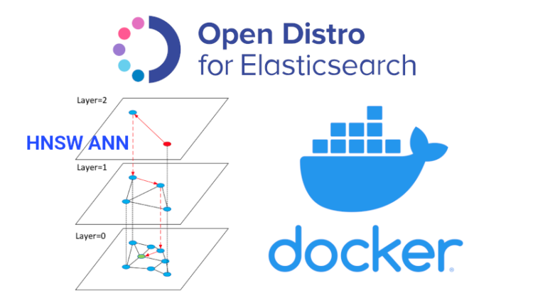
- Scalable ANN: OpenDistro ES distribution has implemented the HNSW ANN algorithm as a plugin [Link]. ES’s distributed nature enables it to scale this high-speed, high-accuracy HNSW ANN search to many millions of records.
- Support: Most modern IT and Infrastructure teams are already familiar with (and heavily using) ES. As a Data Scientist, you probably want the IT Infra team to set up and maintain the server hardware, so using a technology that they are already familiar with increases your chance of securing their support. This support can literally make or break the productionizing of your Data Science project, so don’t underestimate it!
- Simpler Stack: ES can be used as a database to store additional fields, which can then be queried together with the nearest neighbors. For example, if you search for nearest neighbors using product name embeddings, you can also get the product price, category, date added, etc. As long as you stored it in ES, you can retrieve it during the ANN search. This simplifies your application stack because you can get all the information you need from one place instead of querying the nearest neighbors from one location and then hitting another database to get the other fields for all these neighbors.
This is super-duper simple using Docker. We’ll follow the instructions from the official documentation [Link].
Important! This setup is only for your experimentation of HNSW ANN on ES! For Production setup, please ask your IT Infra team to set up the necessary security protocols.
Single Machine
- Install
dockeron your machine following instructions from the docker website [Link] - Pull the docker image for OpenDistro:
sudo docker pull amazon/opendistro-for-elasticsearch:1.12.0 - Run the docker image:
sudo docker run --rm -p 9200:9200 -p 9600:9600 -e "discovery.type=single-node" amazon/opendistro-for-elasticsearch:1.12.0
That’s it! You can now interact with the ES service.
A Cluster of Multiple Machines
Run the following steps in each of the machines you want to set up in your cluster. Again Important! This is just for experimentation, DO NOT use it in production without the proper security protocols.
- Install
dockeron each of your machines following instructions from the docker website [Link] - Pull the docker image for OpenDistro on each of your machines:
sudo docker pull amazon/opendistro-for-elasticsearch:1.12.0 - Install
docker-composefollowing instructions from the docker website [Link] - Create a
docker-compose.ymlfile - Create a
elasticsearch.ymlfile - Start the ES service:
sudo docker-compose up
For example docker-compose.yml and elasticsearch.yml, take a look at my Github repository.
If you encounter any errors, try updating the VM map count as per [Link]: sudo sysctl -w vm.max_map_count=262144.
Check ES Status
After you complete running the steps above on each of your machines, you can check the status of your cluster by using: curl -XGET <ip_address_of_any_node>:9200/_cat/nodes?v -u <username>:<password> —- insecure. You should see all the nodes in your cluster.
Open a DataFrame to load into ES.
We shall use the same Amazon 500K product dataset used in my previous post KNN is Dead!
import pandas as pd
df = pd.read_pickle("df.pkl")
embedding_col = "emb"print(df.shape)
df.head()
Creating an ES Index with HNSW
Once you have setup OpenDistro ES, we need to create an ES Index that will hold all our data. This can be done either by using the Python requests library or using the Python ElasticSearch library: pip install elasticsearch. I’ll use the ElasticSearch library in this post.
In this step, we need to specify the HNSW parameters ef_construction and M as part of the ES index settings. We also need to indicate whether to use l2 (euclidean) or cosinesimil (angular) distance to find neighbors. Some of the settings are best practices from [Link]
# Imports
from elasticsearch import Elasticsearch# ES constants
index_name = "amazon-500k"es = Elasticsearch(["<ip_address_of_any_node>:9200"],
http_auth=(<username>, <password>),
verify_certs=False)# ES settings
body = {
"settings": {
"index": {
"knn": True,
"knn.space_type": "l2",
"knn.algo_param.ef_construction": 100,
"knn.algo_param.m": 16
},
"number_of_shards": 10,
"number_of_replicas": 0,
"refresh_interval": -1,
"translog.flush_threshold_size": "10gb"
}
}mapping = {
"properties": {
embedding_col: {
"type": "knn_vector",
"dimension": len(df.loc[0,embedding_col])
}
}
}# Create the Index
es.indices.create(index_name, body=body)
es.indices.put_mapping(mapping, index_name)
After you complete running the code above, we can check the available indices on our ES cluster using : curl -XGET <ip_address_of_any_node>:9200/_cat/indices?v -u <username>:<password> —- insecure
Uploading Data
Now that the index has been created, we can upload data to it either by using the Python requests library or using the Python ElasticSearch library, which is shown below.
# Imports
from elasticsearch.helpers import bulk
from tqdm import tqdm# Data Generator
def gen():
for row in tqdm(df.itertuples(), total=len(df)):
output_yield = {
"_op_type": "index",
"_index": index_name
}
output_yield.update(row._asdict())
output_yield.update({
embedding_col: output_yield[embedding_col].tolist()
})    yield output_yield# Upload data to ES in bulk
_, errors = bulk(es, gen(), chunk_size=500, max_retries=2)
assert len(errors) == 0, errors# Refresh the data
es.indices.refresh(index_name, request_timeout=1000)# Warmup API
res = requests.get("<ip_address>:9200/_opendistro/_knn/warmup/"+index_name+"?pretty", auth=(<username>, <password>), verify=False)
print(res.text)
Querying Nearest Neighbors
Once we have uploaded all our data into the ES index, we can then query the “K” nearest neighbors for any new data point as follows.
# Query parameters
query_df = <dataframe of items to query, same schema as df>
K = 5 # Number of neighbors
step = 200 # Number of items to query at a time
cols_to_query = ["Index", "title"]# Update the search settings
body = {
"settings": {
"index": {"knn.algo_param.ef_search": 100}
}
}es.indices.put_settings(body=body, index=index_name)# Run the Query
responses = []
for n in tqdm(range(0, len(query_df), step)):
subset_df = query_df.iloc[n:n+step,:]
request = []for row in subset_df.itertuples():
request.extend([req_head, req_body]) r = es.msearch(body=request)
req_head = {"index": index_name}
req_body = {
"query": {
"knn": {
embedding_col: {
"vector": getattr(row, embedding_col).tolist(),
"k": K
}
}
},
"size": K,
"_source": cols_to_query
}
responses.extend(r['responses'])# Convert the responses to dataframe columns
nn_data = {f'es_neighbors_{key}': [] for key in cols_to_query}for item in tqdm(responses):
nn = pd.concat(map(pd.DataFrame.from_dict,
item['hits']['hits']),
axis=1)['_source'].T.reset_index(drop=True)
for key in cols_to_query:
nn_data[f'es_neighbors_{key}'].append(nn[key]
.values
.tolist())query_df = query_df.assign(**nn_data)
query_df.head()
Let’s take a closer look at the neighbors for one of the rows in query_df. They’re all phone cases for the same phone indicating just how good the nearest neighbor search is!
query_df["es_neighbors_title"].iloc[0]
Deleting an ES Index
Finally, after our experimentation is done (or if we made a mistake and need to delete everything to start from scratch), we can delete the whole index with a single line of code as below.
es.indices.delete(index=index_name)