The goal of this article is to demonstrate a model, using physics based feature engineering, that can identify different types of floors (i.e. concrete, wood, carpet etc.) using data collected from Inertial Measurement Units (IMU sensors). The data was collected while driving a small robot on different types of floors.
Different features from the data are generated based on the physics based model of the system, especially the equations of motions, as well as the control system response of the robot as it travels over different surface type. This data is then used to create model using Random Forest Classifier.
This notebook highlights the new features that are used, the rationale behind the decisions and the improvements that are observed.
There are other existing notebooks on the Kaggle website that use Random Forest Classifier to predict floor types. However, in this article, different features are used and these features are selected based on the physics based model of the robot. The parameters of the classifier are tuned to investigate the effects on the accuracy of the model as well.
Some notebooks on the Kaggle website provides aesthetically pleasing data visualization tools. Some of these tools are used here to visualize the data during the data exploration phase.
In this section, the data is explored to create a feature generation strategy. We begin by importing some useful libraries in python.
Now, the data is loaded for exploration
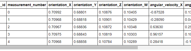
Let’s look at which training features are available from the very beginning. The first and the second table shows the first 10 rows of the training and test data respectively. The complete tables are presented here.
Visual Inspection
Each feature in the training and test data is plotted to visually compare both of the sets. Both sets seems to be similar with no obvious outliers. This is done prior to making a model to eliminate the possibility of bad test data.
Some important information is provided in the challenge description. For example, each measurement series has an unique ID and contains 128 measurements from 10 sensors (features). Each measurement also has an unique number within the series. This information will be used in the feature generation phase.
We now plot the data from a randomly chosen series to visually determine if there are any strong correlations among the features. We see that both orientation_X and orientation_Y decrease simultaneously. There are no other obvious patterns in the plots, but please note the cyclic nature of the angular velocities. This was one of the key information used in feature generation.
The correlation between orientation_X and orientation_Y that was observed in time series 10, does that exist across all the series? Let’s find out how many unique series are in the training set.
3790
If we wanted to visually inspect and find correlations in every time series, we have to inspect 3790 plots. That is a lot of plots! Let’s look at the correlation matrix of the entire training set instead.
We see that the same strong correlation between orientation_X and orientation_Y in the time series 10 is very weak throughout training set. There are, however, strong correlations between the angular_velocity_Y and angular_velocity_Z, and linear_acceleration_Y and lineary_acceleration_Z.
We know that a spinning top becomes unstable when its angular velocity decreases. Is it possible that the robot becomes unstable (an increase in the angular_velocity_Z) as it slows down from a turn (a decrease in the angular_velocity_Y)? The correlation between the linear_acceleration_Y and linear_acceleration_Z is not very strong, but still there.
According to this post, there is a strong correlation between the quaternions and the surface type. We have seen that there is strong correlation between angular velocities (Y and Z) and a cyclic pattern in the angular velocities. Are we dealing with a self balancing robot, that is trying to balance itself on different surface type as it drives around. If so, the orientation of the robot might be coupled to the surface type via friction (i.e. different coefficients of friction).
In the following sections we will generate additional features after examining the equations of motion that govern the inverted pendulum system (related to Segway, booster rocket control system etc.). Inverted pendulum model has also been used to understand bipedal (human walking) motion. We will also remove the quaternions in order eliminate any direct effect on prediction accuracy.
We will change the quaternions to the roll, pitch and yaw. The function below also return the sine and cosine of each of the angle, but the rationale behind these features will be given later.
We now look at the distribution of the features across each surface type. We ignore the quaternions and focus on the roll, pitch and yaw instead. The function below plots each feature across different floors on each of the subplots.
We see that, based on the distribution curves, different components (X,Y and Z) of the linear acceleration, angular velocity along with the calculated pitch (euler_z) and sin(z) migh have the biggest impact on the prediction. The distribution of the euler_z seems to indicate that the robot might have been trying to balance itself differently on different surface (i.e. the effect of friction on the balance was different for each floor type). To find out if it is indeed a possibility, we look at the equations of motion that govern an inverted pendulum system in the following section.
Note: I have yet to find an easier way of writing mathematical notation in medium. So, I am going to reproduce some sections from Google Colab. You can read the whole section here as well.
A detailed description of the inverted pendulum system can be found here.
In the last section we showed that the orientation of the center of mass of the robot and the its linear acceleration might be very useful features. However, does our data conform to this inverted pendulum model. Before moving on, we make some assumptions — we don’t know the mass, geometric features of the robot or anything about the control system parameters. We assume that the data that is available to us is collected from an IMU located at the center of mass of the robot, i.e. the orientation, angular velocity and linear accelration data describe the state of the robot’s center of mass.
To find out if the data does indeed conform to the inverted pendulum model presented here, we plot the orientation of the robot on different surface types. If the robot was actively balancing itself then the pitch, roll and yaw will be constrained within a narrow range. The figures below show that the range of the orientation on concrete is indeed narrow. Though it is not shown, the range of the orientation is also narrow for other surface types.
In the figure above, we see that the orientation of the robot is changing frequently between a narrow range. Recall that we saw the cyclic pattern in the angular velocities in the data exploration section, which is linked to the frequent change in orientation seen here. We may have some evidence to believe that we are dealing with a self balancing robot that is actively trying to balance itself as it drives across different surfaces.
Since there is some evidence that the robot is trying to actively balance itself, one can ask the following question — is it possible to use the control system’s response to identify the surface type i.e. does the control system react differently to different surface? It should, if the surface characteristics (roughness or friction) of each surface are drastically different.
With this in mind, we will analyze the roll, pitch and yaw to determine how frequently these change and these will be added to the list of features. The idea is that for different surface type the frequency will be different. The following functions use Fast Fourier Transform to determine the frequency with the largest and amplitude.
We also use the information about the distribution of each given feature on different surfaces as new features. This is done to create a feature that uniquely describes a surfaces. For example, it may help us to find out if the maximum total angular velocity differs across surface types and we can use that to differentiate between surfaces.
We use the mean, median, standard deviation, maximum, minimum, range, ratio between maximum to minimum, average change etc. of each feature to create an unique characteristic (signature) of each surface type. We do this by aggregating the data by series ID since we know that the relationship between surface type and a series ID is 1:1 (given in the data description).
The following function is used to generate the new features.
As promised, before we generate new features, we remove the quaternions from the training and testing sets completely. We use the following for that purpose.
We check the training and test set to verify that the quaternions have indeed been removed from the sets.
Once again, you can see the full tables here.
Now we generate the new features using the function described previously.
Random Forest Classifier works well with non-linear features and features that are highly similar to each other. Our features are also on various scales and Random Forest work well with this kind of features too. We don’t know anything about the precision and the accuracy of the IMU. Random Forest Classifier is robust with respect to noisy data. In the following section, we briefly describe the Random Forest Classifier.
Random Forest Classifier
Random Forest Classifier is an ensemble of larger number of individual decision trees. Each individual tree returns a class prediction and the class with most votes is the final prediction. Since there is low correlation between the trees, the predictions are more accurate. Each tree implements a recursive binary partition of the input feature space. The partition occurs based on tests that involves the features and the corresponding threshold values.
Since, we are already using features that are aggregated characteristics of each original features i.e. mean angular velocity, max angular velocity, max frequency of change in orientation etc. for each floor type over several time series, these features when taken together create an unique signature for each surface type. When measured across several time series for a given surface type, these signatures should be located very close to each other (considering error propagation from the accuracy and precision of the IMU). Using a Random Forest Classifier will be a good option since the feature space can be partitioned easily.
Before we can begin training the model we need to convert the name of the surfaces (categorical text data) to numerical data. For example, map “concrete” to 1, “carpet” to 2 etc.
Next, we replace infinities, and NaN values with zeroes. We do this in the case some of the results of the feature generation are the former values.
The following are used to check if there are any very large values in the training or test sets.
I didn’t find any large values, please feel free to check my work.
To train the model we split the training set into several training and cross validation sets using the Scikit-learn StratifiedKFold() function. The training and test set, after the feature generation stage, no longer contain any time series, but only the unique signatures for each surface type (discussed previously). As such, this splitting strategy should not be prone to data leak due to temporal dependency discussed here.
Then we fit the model and determine the model accuracy on the cross validation set. For each model, we predict the surface type probability (divided by the number of splits since the split is random and we do not have the complete feature distribution of the entire set at each model fitting) based on the test data set. Ultimately, we choose the maximum probability of each surface type from the set model predictions.
Let’s run the model and see how it performs.
The accuracy on the training set is 0.89, but is it an improvement? In the Appendix, there are results based on feature sets where the quaternions, roll, pitch, yaw, frequency of angle change are missing. These are the features that had been added based on the equations of motion of the inverse pendulum system. The accuracy of 0.89 is a significant improvement over 0.59 without the features. Even if we add just the rotation about the Z-axis and the associated frequency of change, the accuracy goes up to 0.82 (shown in the Appendix).
Tuning the Hyperparameters
We have seen the improvements due to the addition of the new features, but can we still make improvements by tuning the hyperparameters such as the number of trees in the forest, number of features considered by a tree node etc.?
We start by finding out the parameters that are currently in used by the random forest classifier model.
From these, we choose the following parameters to modify.
Now, we use RandomSearchCV() to find best parameters from the grid. RandomSearchCV() randomly samples a grid of predefined hyperparameter ranges and performs K-Fold cross validation with each combination of values.
Now we train our model with the updated parameters.
Well it doesn’t look like the accuracy has increase too much (still 0.89) and we are still using the training set. Let’s compare the output of each and the provided test labels.
The following shows the prediction difference between the model with tuned parameter vs model without parameter tuning.
I found no difference between the models (please feel free to check my work). So we can use any of these two for cross validation.
Looks like our untuned model has misclassified one surface type out of 20.
After observing the model performance, it can be said that the features selected based on the equation of motion resulted in better prediction. There is still room for improvements, for example we could have investigated hyperparameter tuning more, but that could result in over fitting.
Here we will present the difference in prediction accuracy with different feature selection. First we look at the feature set that does not include the quaternions or any other features based on the equations of motion.