In the last week, we took a plunge into the core concepts of Deep Learning and the framework of a Neural Network. We also touched upon the basics of an objective function and its use, the kinds of objective functions and how Gradient Descent plays a pivotal role in rectifying the mistakes/error while predicting a value.
In this article, we shall feast our mind and thought on Autoencoders.
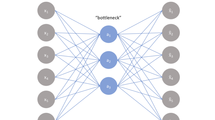
Starting off , let’s have a look at what Autoencoders are. Most of you would be aware of the basic form and structure of a neural network. An auto encoder is a neural network with an induced bottleneck. This bottleneck force a compressed knowledge representation of the original input data. Autoencoders are very efficient and a great adage in cases where the input data might have certain structures or correlations between them. Correlations help in forcing the input through a network’s bottleneck.
As seen from the above picture, let’s assume we have an unlabeled dataset. We can take this to be basic supervised learning situation and task it with producing an output called x^. This network can be trained by minimizing the reconstruction error, L(x,x^)L(x,x^). Without a bottleneck, the network just memorizes what was passed and relays it as output with no reconstruction whatsoever.
A bottleneck is quite necessary here as it contains the certain amount of information that can traverse the entire network by forcing a learned compression of the inputs provided. The ideal autoencoder will also encompass a loss function which takes into account the reconstruction loss and accordingly adds a regulariser that discourages overfitting or memorization. Let’s have a look at the kinds of autoencoding structures.
The simplest architecture for constructing an autoencoder is to ensure a limit on the number of nodes present in the hidden layer of the neural network. By penalizing the network according to the reconstruction error that we’d have calculated, the model would be able to list down the more important variables/attributes and how to reconstruct the input from an encoded state ( during the output phase ).
Because networks are capable of establishing non-linear relationships, this will immediately strike as a powerful PCA technique. PCA aims to discover a lower dimensional hyper plane, whereas an autoencoder are capable enough to learn from non-linear manifolds. What’s a manifold? A manifold is a continuous non-intersecting surface. We can understand this better by having a look at this representation.
An undercomplete autoencoder does not possess an explicit regularization function. The model is trained off the reconstruction loss ( computed earlier ). To hence ensure that the model does not memorize any of the input data, is to sufficiently restrict the number of nodes in the hidden layer of this autoencoder. One needs to also understand that the sole purpose of an autoencoder is to not just restrict memorization, but to also bring out the hidden latent attributes within the data. As done in a supervised learning model, regularization can be applied in different ways to extract attribute relationships better.
Unlike undercomplete autoencoders, sparse autoencoders introduce a method to introduce an information bottleneck without having to reduce the number of nodes in the hidden layer. The loss function is designed in such a way so as to penalize certain activations in a layer.
What that means is, for every data bit that is decoded, the network will be encouraged to activate a certain set of neurons. One must note that, as opposed to a regular neural network, where we update the weights, in sparse autoencoders, the activations are being updated. Note that, the individual nodes of a trained model which get activated, are dependent on the kind of data parsed. Different inputs will result in activations of different nodes through the network.
A sparse autoencoder is forced to selectively activate certain neurons only, as opposed to the entire network in undercomplete autoencoder. This, in turn, reduces the network’s ability to memorize data is reduced to a greater extent.
This sparsity constraint is imposed by measuring the hidden layer activations for each training group and adding terms to loss function in order to penalize excessive activations. The terms are :
- L1 Regularization :
This term is added to the loss function that penalizes the values of a vector of activations “a” in some hidden layer “h” for some observation “i” with a tuning parameter lambda.
2. KL-Divergence
This is a measure of the difference between two probability distributions. We define a sparsity parameter which denotes the average activation of a neuron over a collection of samples. This can be calculated as :
j — indicates the specific neuron in a layer “h”, summing the activations for “m” training observations denoted by x. We can describe ρ as a Bernoulli random variable here. Hence, if we put the two comparisons together, we have :
There are a couple of other types of autoencoders, do let us know if you need an article on those 2 🙂
An autoencoder is a network capable of determining structures and correlations within data and can develop a compressed interpretation of the same. The biggest challenge with autoencoders lies in the fact that one needs to train it to extract meaningful inferences from data. These models are capable enough to only reconstruct data similar to the class of observations that it observed during a training process.
