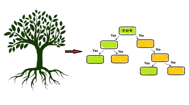
In-depth study of decision tree for classification problem
In this article, the decision tree algorithm is the base model for all other tree models. The decision tree comes in the CART (classification and regression tree) algorithm that is an optimized version in sklearn. These are non-parametric supervised learning. The non-parametric means that the data is distribution-free i.e the variables are nominal or ordinal.
The decision tree decides by choosing the root node and split further into nodes. The splitting is based on metrics used in the decision tree. The earlier article was on metrics of regression and classification. But in the case of a decision tree, the metrics are a little bit different.
Metrics in the decision tree
- Gini Impurity and Entropy
- Information Gain
- Variance Reduction
The decision tree has a few types of an algorithm that generate decision tree from the dataset as shown below:
- ID3 (iterative dichotomiser 3): It generates smaller trees and not useful on continuous data because it causes to find multiple split in that attribute and takes a longer time. It is also do overfit on the training set.
- C4.5: It is an advanced version of ID3 that also work on continuous data based on a threshold value. It is also useful in a dataset with missing values. After the creation of trees, it can do pruning also.
- CART: It is a classification and regression tree that generate trees based on whether the output variable is categorical or numerical. The CART detects no further gain is possible in the attribute and stops splitting.
We will see how different algorithm uses a different metric to do the splitting of trees.
Gini and Entropy
- Gini impurity is used in the CART version of the algorithm. It is used to find the probability of misclassifying observations and better splitting is done with a lower number of Gini value.
- The entropy is also used for splitting the trees based on misclassifying observations. It takes a little longer time because of the log computation.
- The main difference here is to notice that Gini takes a range from 0 to 0.5. While entropy takes a range from 0 to 1.
- Entropy is used in the ID3 and C4.5 versions of the algorithm.
Information Gain
It is used with the entropy value. The difference in the value of entropy from the prior state to the information state.
In general, the splitting is done based on maximum gain or information from the target variable to the other attribute.
Gain(i) = Information gain(Y)-entropy(Ai)
Y — Dependent variable
Ai — Attributes of an independent variable (i=1,2…n)
Variance Reduction
It is useful in regression problems because the splitting of the node is based on variance value when the output variable is in continuous numbers.
Now it’s time to do practical with python for classification problems.
# Importing the libraries
import numpy as np
import matplotlib.pyplot as plt
import pandas as pd
The next step after importing the libraries now we will read the CSV file and dividing the data into features and target variables.
# Importing the dataset
dataset = pd.read_csv('Social_Network_Ads.csv')
x_set_values = dataset.iloc[:, [2, 3]].values
y_set_values = dataset.iloc[:, 4].values
Now divide the data into training and testing data.
# Splitting the dataset into the Training set and Test set
from sklearn.model_selection import train_test_splitX_train, X_test, y_train, y_test = train_test_split(x_set_values,
y_set_values, test_size = 0.25, random_state = 0)
In the next step, we can do standard scaling but I think that in the decision tree we should not do that because the splitting should be based on real values not on scaled values. But in case the scaling part is given below:
#Feature Scaling
from sklearn.preprocessing import StandardScaler
sc = StandardScaler()
X_train = sc.fit_transform(X_train)
X_test = sc.transform(X_test)
In this algorithm, we will use Entropy.
# Fitting the classifier classifier to the Training set
from sklearn.tree import DecisionTreeClassifier
classifier = DecisionTreeClassifier(criterion = 'entropy', random_state= 0)
classifier.fit(X_train, y_train)#output:DecisionTreeClassifier(class_weight=None, criterion='entropy',
max_depth=None,
max_features=None, max_leaf_nodes=None,
min_impurity_decrease=0.0, min_impurity_split=None,
min_samples_leaf=1, min_samples_split=2,
min_weight_fraction_leaf=0.0, presort=False,
random_state=0,splitter='best')
Now, we will predict the data and make our model.
# Predicting the Test set results
y_pred = classifier.predict(X_test)
Now, we compute the confusion matrix.
# Making the Confusion Matrix
from sklearn.metrics import confusion_matrix
cm = confusion_matrix(y_test, y_pred)
#output:array([[66,  2],
[ 8, 24]], dtype=int64)
To visualize the training and testing result with Entropy.
# Visualising the Training set results
from matplotlib.colors import ListedColormapX_set, y_set = X_train, y_trainX1, X2 = np.meshgrid(np.arange(start = X_set[:, 0].min() - 1, stop =
X_set[:, 0].max() + 1, step = 0.01),
np.arange(start = X_set[:, 1].min() - 1, stop =
X_set[:, 1].max() + 1, step = 0.01))plt.contourf(X1, X2, classifier.predict(np.array([X1.ravel(),
X2.ravel()]).T).reshape(X1.shape),
alpha = 0.5, cmap = ListedColormap(('red', 'green')))plt.xlim(X1.min(), X1.max())
plt.ylim(X2.min(), X2.max())for i, j in enumerate(np.unique(y_set)):
plt.scatter(X_set[y_set == j, 0], X_set[y_set == j, 1],
alpha=0.5,
c = ListedColormap(('red', 'green'))(i), label = j)plt.title('Decision Tree (Training set)')
plt.xlabel('Age')
plt.ylabel('Estimated Salary')
plt.legend()
plt.show()
After changing the criterion to ‘Gini’ doesn’t change the confusion matrix value.
These are tree splitting separation criterion with entropy and Gini on training set. We observe that there is good classification in the graph.
Conclusion:
The Decision tree is very useful in classification and regression. The criterion parameter gives different tree splitting of data set.
I hope you like the article. Reach me on my LinkedIn and twitter.
- NLP — Zero to Hero with Python
2. Python Data Structures Data-types and Objects
3. Python: Zero to Hero with Examples
4. MySQL: Zero to Hero
5. Basics of Time Series with Python
6. NumPy: Zero to Hero with Python
7. Fundamentals of series and Data Frame in Pandas with python
8. Confusion Matrix in Machine Learning
