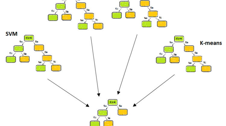
The machine learning methods based on several decision trees
In this article, The ensemble techniques are based on multiple decision trees. If we talk about only the decision tree that gives high variance after modeling which leads to over-fitting. The benefit of using ensemble methods is giving good prediction with reduced variance by averaging(bagging) or by boosting techniques.
There are various types of ensemble techniques likes classification and regression as shown below:
- Bagging, Random forest and Extra trees are in averaging methods.
- Adaboost, Gradient boosting, CatBoost, etc are in boosting methods.
In averaging methods, usually used to reduce the variance while the final prediction is made on the average value of all other weak learners or base learners. Here base learners are the different algorithms used to make predictions.
We use bootstrapping sampling dataset of the same shape as the original to all others with replacement so that, the prediction from all the models would not be the same.
In boosting methods, usually used to reduce the bias while the prediction is based on sequential wise, means the error from first taken by the next model with improved prediction and so on till the last base model.
In this article, we will discuss random forest algorithms with python implementation and others will be in future subsequent articles.
The sklearn have two flavors of random forest i.e. RandomForestClassifier and RandomForestRegression
These two flavors have different criterion parameter also as shown below:
- Random classifiers have
giniandentropymetrics and the default is Gini. - Random regression has
MSEandMAEmetrics i.e. mean squared error and mean absolute error while here the default is MSE.
The other parameters are also useful like n_estimator and max_features. The default value of the former is 100 (i.e 100 decision trees) and but it is better with more number of estimators till significant. While the latter one is the size of the random subset for the best split.
If the number of max_features increases it may cause more bias and with less number, there is a good reduction in variance.
The other noticeable parameter is n_jobs it means if we want to do fast processing then we have to put the value to “-1” other than the default is none. This process is known as parallelization in which the machine will use all the cores for multiprocessing.
The default value of bootstrap is true.
The Python implementation with regression and classification is shown below:
Now we will do a practice to solve the classification problem with SVM.
With Classification
# Importing the libraries
import numpy as np
import matplotlib.pyplot as plt
import pandas as pd
After importing the libraries now we will read the CSV file and dividing the features into independent and dependent variables.
# Importing the dataset
dataset = pd.read_csv('Social_Network_Ads.csv')
x_set_values = dataset.iloc[:, [2, 3]].values
y_set_values = dataset.iloc[:, 4].values
Now dividing the data set into training set and testing set.
from sklearn.model_selection import train_test_splitX_train, X_test, y_train, y_test = train_test_split(x_set_values,
y_set_values, test_size = 0.25, random_state = 0)
Before modeling the machine learning algorithm we should always do the standard scaling.
# Feature Scaling
from sklearn.preprocessing import StandardScaler
sc = StandardScaler()
X_train = sc.fit_transform(X_train)
X_test = sc.transform(X_test)
In this algorithm, we will use a entropy criterion.
# Fitting the classifier to the Training set
from sklearn.ensemble import RandomForestClassifierclassifier = RandomForestClassifier(n_estimators = 10, criterion =
'entropy', random_state= 0)classifier.fit(X_train, y_train)#output:RandomForestClassifier(bootstrap=True, class_weight=None,
criterion='entropy', max_depth=None, max_features='auto',
max_leaf_nodes=None, min_impurity_decrease=0.0,
min_impurity_split=None, min_samples_leaf=1,
min_samples_split=2, min_weight_fraction_leaf=0.0,
n_estimators=10, n_jobs=None, oob_score=False, random_state=0,
verbose=0, warm_start=False)
Now, we will predict the data and make our model.
# Predicting the Test set results
y_pred = classifier.predict(X_test)
Now, we compute the confusion matrix.
# Making the Confusion Matrix
from sklearn.metrics import confusion_matrix
cm = confusion_matrix(y_test, y_pred)#output:
array([[63,  5],
[ 4, 28]], dtype=int64)
To visualize the training and testing result with Entropy Criterion.
# Visualising the Training set results
from matplotlib.colors import ListedColormapX_set, y_set = X_train, y_trainX1, X2 = np.meshgrid(np.arange(start = X_set[:, 0].min() - 1, stop =
X_set[:, 0].max() + 1, step = 0.01),
np.arange(start = X_set[:, 1].min() - 1, stop =
X_set[:, 1].max() + 1, step = 0.01))plt.contourf(X1, X2, classifier.predict(np.array([X1.ravel(),
X2.ravel()]).T).reshape(X1.shape),
alpha = 0.5, cmap = ListedColormap(('red', 'green')))plt.xlim(X1.min(), X1.max())
plt.ylim(X2.min(), X2.max())for i, j in enumerate(np.unique(y_set)):
plt.scatter(X_set[y_set == j, 0], X_set[y_set == j, 1],
alpha=0.5, c = ListedColormap(('red', 'green'))(i),
label = j)plt.title('Random Forest Classifier (Training set) with Entropy')
plt.xlabel('Age')
plt.ylabel('Estimated Salary')
plt.legend()
plt.show()
Change for testing set
X_set, y_set = X_test, y_testand plt.title('Random Forest Classifier (Testing set) with Entropy')
