GoogLeNet (InceptionV1) with TensorFlow

InceptionV1 or with a more remarkable name GoogLeNet is one of the most successful models of the earlier years of convolutional neural networks. Szegedy et al. from Google Inc. published the model in their paper named Going Deeper with Convolutions[1] and won ILSVRC-2014 with a large margin. The name both signifies the affiliation of most of the contributed scholars with Google and the reference to the LeNet[2] model.

For the previous posts, please visit:

Introduction

After analyzing and implementing VGG16[7] (runner-up of ILSVRC-2014), now it is time for the winner of the competition, GoogLeNet. As the name of the paper[1] implies the main intuition of GoogLeNet is obtaining a more capable model by increasing the dept. However, as covered in the previous posts, it is a risky architectural choice since deeper and larger models are notoriously harder to train. The success of GoogLeNet stems from the smart tricks that make the model lighter and easier to train. The original GoogLeNet is also named InceptionV1 and it is a 22-layers-deep network. Other versions of the model have also been developed by some of the writers of the first paper in 2016[3].

A few new ideas made GoogLeNet superior to the counterpart model VGGNet:

1. 1×1 convolutions were used for reducing the dimensionality of the layers while making the model deeper.
2. Average global pooling[6] is performed before the fully connected layers in order to reduce the number of feature maps.
3. Two auxiliary losses were introduced at the earlier layers of the model for the sake of propagating good gradients to the initial layers. It is a very brilliant idea for tackling the vanishing gradient problem.
4. Prior models such as LeNet, AlexNet, and VGGNet follow a sequential model architecture. However, GoogLeNet has braches that lead to auxiliary losses.
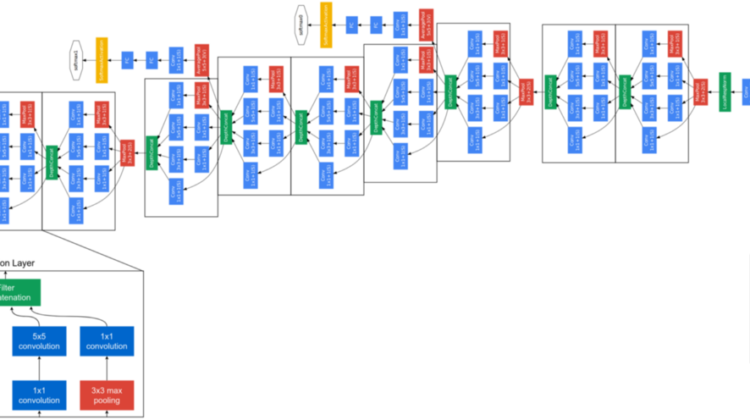
5. Another branchy entity in the model is the Inception module that combines the outputs of differently sized filters. The parallel structure of multiple scales enables the module to capture both smaller and larger motifs in the pixel-data.

All these ideas will be discussed further throughout the next sections as we build the model using Keras.

This tutorial is intended for beginners to demonstrate a basic TensorFlow implementation of GoogLeNet on the MNIST dataset. For more information on CNNs and TensorFlow, you can visit the previous posts linked at the beginning of this article. The reason for the usage of MNIST instead of ImageNet is simplicity, but the model can be used for any dataset with very few variations in the code.

First, needed libraries are imported.

import tensorflow as tf
import matplotlib.pyplot as plt
from tensorflow.keras import datasets, layers, models, losses, Model

The Data

Then, the data is loaded as in the LeNet implementation. One important notice is that the original GoogLeNet model receives images with the size 224 x 224 x 3 however, MNIST images are 28 x 28. The third axis is expanded and repeated 3 times to make image sizes 28 x 28 x 3. It will be then resized at the first layer of the model to 224 x 224 x 3.

(x_train,y_train),(x_test,y_test) = datasets.mnist.load_data()
x_train = tf.pad(x_train, [[0, 0], [2,2], [2,2]])/255
x_test = tf.pad(x_test, [[0, 0], [2,2], [2,2]])/255
x_train = tf.expand_dims(x_train, axis=3, name=None)
x_test = tf.expand_dims(x_test, axis=3, name=None)
x_train = tf.repeat(x_train, 3, axis=3)
x_test = tf.repeat(x_test, 3, axis=3)
x_val = x_train[-2000:,:,:,:]
y_val = y_train[-2000:]
x_train = x_train[:-2000,:,:,:]
y_train = y_train[:-2000]

The Model

GoogLeNet is a deep network and used this advantage to come on top of the ImageNet classification challenge in 2014. But why other researchers did not design their models even deeper than GoogLeNet and achieve higher accuracies? The answer is that there is no direct correlation between the dept of the model and the accuracy it yields in certain tasks. Mostly, there is a sweet spot for the size of the networks, and if it is exceeded it becomes really cumbersome, sometimes infeasible, to train the models. There are two aspects of this problem:

1. Deeper networks mean more parameters to be trained, which requires an abundance of data, clever ways of training procedures, and most importantly strong GPUs. The available data and hardware enabled larger and larger networks nowadays, yet that was not the case back in time. GoogLeNet uses 1×1 convolutions to reduce the number of feature maps and deepen the network while preserving the image sizes and not introducing many parameters.
2. During the propagation, gradients are calculated in terms of the losses and they flow back from the prediction layer to the initial layer. In deeper networks, gradients have to traverse a long way and go through several operations. A common problem is that these gradients get smaller and smaller as they get multiplied with activations between 0 and 1. Also, unbounded activations may blow up the gradients, which poses a similar problem. GoogLeNet introduces two auxiliary losses before the actual loss and makes more sensible gradients flow backward. So, these gradients travel a shorter path and help initial layers converge faster.

These two approaches enabled GoogLeNet to be deeper and as it gets deeper its learning capacity also increases which leads to higher accuracies.

Another trick is the use of global average pooling. Convolutional networks are superior to multilayer perceptrons in terms of efficiency thanks to the weight sharing[6] mechanism. However, for classification purposes, fully connected layers are added at the top of the models and they are usually responsible for most of the parameters in the network. GoogLeNet reduces the number of neurons by taking an average among the channels right before the dense layer.

The parallel flow of the information is another key factor in the success of GoogLeNet. Patterns with different scales get captured and stacked on top of each other. A parallel backpropagation is also efficient compared to a sequential order since the gradients do not suffer vanishing/exploding. 1×1 convolutions control the feature map sizes.

The inception model is coded as follows:

def inception(x,
filters_1x1,
filters_3x3_reduce,
filters_3x3,
filters_5x5_reduce,
filters_5x5,
filters_pool):  path1 = layers.Conv2D(filters_1x1, (1, 1), padding='same',    activation='relu')(x)  path2 = layers.Conv2D(filters_3x3_reduce, (1, 1), padding='same', activation='relu')(x)
path2 = layers.Conv2D(filters_3x3, (1, 1), padding='same', activation='relu')(path2)  path3 = layers.Conv2D(filters_5x5_reduce, (1, 1), padding='same', activation='relu')(x)
path3 = layers.Conv2D(filters_5x5, (1, 1), padding='same', activation='relu')(path3)  path4 = layers.MaxPool2D((3, 3), strides=(1, 1), padding='same')(x)
path4 = layers.Conv2D(filters_pool, (1, 1), padding='same', activation='relu')(path4)  return tf.concat([path1, path2, path3, path4], axis=3)

A big thanks to the blog post[5] by Faizan Shaik who share some code snippets that were very useful when I was coding this model.

The rest of the model is carefully built by following the figure at the top of this article. Inception modules, auxiliary outputs, and subsampling layers were all placed in the correct order.

inp = layers.Input(shape=(32, 32, 3))input_tensor = layers.experimental.preprocessing.Resizing(224, 224, interpolation="bilinear", input_shape=x_train.shape[1:])(inp)x = layers.Conv2D(64, 7, strides=2, padding='same', activation='relu')(input_tensor)
x = layers.MaxPooling2D(3, strides=2)(x)x = layers.Conv2D(64, 1, strides=1, padding='same', activation='relu')(x)
x = layers.Conv2D(192, 3, strides=1, padding='same', activation='relu')(x)
x = layers.MaxPooling2D(3, strides=2)(x)x = inception(x, filters_1x1=64, filters_3x3_reduce=96, filters_3x3=128, filters_5x5_reduce=16, filters_5x5=32, filters_pool=32)x = inception(x, filters_1x1=128, filters_3x3_reduce=128, filters_3x3=192, filters_5x5_reduce=32, filters_5x5=96, filters_pool=64)x = layers.MaxPooling2D(3, strides=2)(x)x = inception(x, filters_1x1=192, filters_3x3_reduce=96, filters_3x3=208, filters_5x5_reduce=16, filters_5x5=48, filters_pool=64)aux1 = layers.AveragePooling2D((5, 5), strides=3)(x)
aux1 =layers.Conv2D(128, 1, padding='same', activation='relu')(aux1)
aux1 = layers.Flatten()(aux1)
aux1 = layers.Dense(1024, activation='relu')(aux1)
aux1 = layers.Dropout(0.7)(aux1)
aux1 = layers.Dense(10, activation='softmax')(aux1)x = inception(x, filters_1x1=160, filters_3x3_reduce=112, filters_3x3=224, filters_5x5_reduce=24, filters_5x5=64, filters_pool=64)x = inception(x, filters_1x1=128, filters_3x3_reduce=128, filters_3x3=256, filters_5x5_reduce=24, filters_5x5=64, filters_pool=64)x = inception(x, filters_1x1=112, filters_3x3_reduce=144, filters_3x3=288, filters_5x5_reduce=32, filters_5x5=64, filters_pool=64)aux2 = layers.AveragePooling2D((5, 5), strides=3)(x)
aux2 =layers.Conv2D(128, 1, padding='same', activation='relu')(aux2)
aux2 = layers.Flatten()(aux2)
aux2 = layers.Dense(1024, activation='relu')(aux2)
aux2 = layers.Dropout(0.7)(aux2) 
aux2 = layers.Dense(10, activation='softmax')(aux2)x = inception(x, filters_1x1=256, filters_3x3_reduce=160, filters_3x3=320, filters_5x5_reduce=32, filters_5x5=128, filters_pool=128)x = layers.MaxPooling2D(3, strides=2)(x)x = inception(x, filters_1x1=256, filters_3x3_reduce=160, filters_3x3=320, filters_5x5_reduce=32, filters_5x5=128, filters_pool=128)x = inception(x, filters_1x1=384, filters_3x3_reduce=192, filters_3x3=384, filters_5x5_reduce=48, filters_5x5=128, filters_pool=128)x = layers.GlobalAveragePooling2D()(x)
x = layers.Dropout(0.4)(x)out = layers.Dense(10, activation='softmax')(x)

The computational graph is structured by indicating the input and outputs (including auxiliary outputs).

model = Model(inputs = inp, outputs = [out, aux1, aux2])

Model is compiled and trained with Adam optimizer and categorical cross-entropy loss for all three outputs. The weighted sum of the losses is adjusted such that auxiliary losses are as important as 0.3 times the actual loss.

model.compile(optimizer='adam', 
loss=[losses.sparse_categorical_crossentropy,
losses.sparse_categorical_crossentropy,
losses.sparse_categorical_crossentropy]
loss_weights=[1, 0.3, 0.3],
metrics=['accuracy'])history = model.fit(x_train, [y_train, y_train, y_train], validation_data=(x_val, [y_val, y_val, y_val]), batch_size=64, epochs=40)...
...
Epoch 40/40 907/907 [==============================] - 148s 163ms/step - loss: 0.0184 - dense_4_loss: 0.0113 - dense_1_loss: 0.0118 - dense_3_loss: 0.0119 - dense_4_accuracy: 0.9961 - dense_1_accuracy: 0.9961 - dense_3_accuracy: 0.9966 - val_loss: 0.0525 - val_dense_4_loss: 0.0321 - val_dense_1_loss: 0.0280 - val_dense_3_loss: 0.0402 - val_dense_4_accuracy: 0.9955 - val_dense_1_accuracy: 0.9970 - val_dense_3_accuracy: 0.9955

The result of the dense_4_loss and dense_4_accuracy is what is important for the evaluation since other auxiliary outputs were just useful during training time and meaningless at forward-passing. After 40 epochs validation accuracy reaches up to 99.55%, which is quite impressive.

fig, axs = plt.subplots(2, 1, figsize=(15,15))axs[0].plot(history.history['loss'])
axs[0].plot(history.history['val_loss'])
axs[0].title.set_text('Training Loss vs Validation Loss')
axs[0].set_xlabel('Epochs')
axs[0].set_ylabel('Loss')
axs[0].legend(['Train','Val'])axs[1].plot(history.history['dense_4_accuracy'])
axs[1].plot(history.history['val_dense_4_accuracy'])
axs[1].title.set_text('Training Accuracy vs Validation Accuracy')
axs[1].set_xlabel('Epochs')
axs[1].set_ylabel('Accuracy')
axs[1].legend(['Train', 'Val'])

model.evaluate(x_test, y_test)313/313 [==============================] - 10s 27ms/step - loss: 0.0516 - dense_4_loss: 0.0299 - dense_1_loss: 0.0335 - dense_3_loss: 0.0388 - dense_4_accuracy: 0.9929 - dense_1_accuracy: 0.9923 - dense_3_accuracy: 0.9918

References

- Szegedy, Christian & Liu, Wei & Jia, Yangqing & Sermanet, Pierre & Reed, Scott & Anguelov, Dragomir & Erhan, Dumitru & Vanhoucke, Vincent & Rabinovich, Andrew. (2014). “Going Deeper with Convolutions”.
- LeCun, Y.; Boser, B.; Denker, J. S.; Henderson, D.; Howard, R. E.; Hubbard, W.; Jackel, L. D. (December 1989). “Backpropagation Applied to Handwritten Zip Code Recognition”. Neural Computation. 1(4): 541–551.
- Szegedy, Christian & Vanhoucke, Vincent & Ioffe, Sergey & Shlens, Jon & Wojna, ZB. (2016). “Rethinking the Inception Architecture for Computer Vision”. 10.1109/CVPR.2016.308.
- https://www.geeksforgeeks.org/understanding-googlenet-model-cnn-architecture/
- https://www.analyticsvidhya.com/blog/2018/10/understanding-inception-network-from-scratch/
- Ott, Jordan & Linstead, Erik & LaHaye, Nick & Baldi, Pierre. (2020). Learning in the machine: “To share or not to share?”. Neural Networks. 126. 10.1016/j.neunet.2020.03.016.
- Simonyan, Karen & Zisserman, Andrew. (2014). “Very Deep Convolutional Networks for Large-Scale Image Recognition”. arXiv 1409.1556.