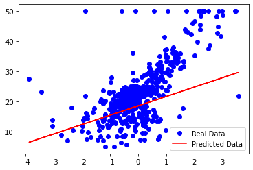
Simple linear regression based on the number of rooms (RM) on the Boston house price dataset.
Our goal is to predict the house price given in the last column (MEDV). Here, we load the dataset from the TensorFlow Contrib dataset directly. We optimize the coefficients for an individual training sample using the stochastic gradient descent optimizer.
- The first step is to import all the packages that we will need:
import numpy as np
import tensorflow as tf
import matplotlib.pyplot as plt
import tensorflow.compat.v1 as tf
tf.disable_v2_behavior()
from sklearn.datasets import load_boston
2. In neural networks, all the inputs are added linearly to generate activity; for
effective training, the inputs should be normalized, so we define a function to
normalize the input data:
def normalize(X):
mean = np.mean(X)
std = np.std(X)
X = (X-mean)/std
return X
3. Now we load the Boston house price dataset using TensorFlow DPOUSJC datasets and separate it into X_train and Y_train. We can choose to normalize the data here:
# databoston = load_boston()X_train, Y_train = boston.data[:,5], boston.targetX_train = normalize(X_train) # this step is optionaln_samples = len(X_train)
4. We declare the TensorFlow placeholders for the training data:
X = tf.placeholder(tf.float32, name ='X')
Y = tf.placeholder(tf.float32, name ='Y')
5. We create TensorFlow variables for weight and bias with initial value zero:
b = tf.Variable(0.0)
w = tf.Variable(0.0)
6. We define the linear regression model to be used for prediction:
Y_hat = X * w + b
7. Define the loss function:
loss = tf.square(Y-Y_hat, name='loss')
8. We choose the gradient descent optimizer:
optimizer = tf.train.GradientDescentOptimizer(learning_rate =0.01).minimize(loss)
9. Declare the initializing operator:
init_op = tf.global_variables_initializer()
total = []
10. Now, we start the computation graph. We run the training for 100 epochs:
with tf.Session() as sess:#initialize variables
sess.run(init_op)
writer = tf.summary.FileWriter('graphs', sess.graph)
#train the model for 100 epochs
for i in range(100):
total_loss = 0
for x,y in zip(X_train, Y_train):
_, l = sess.run([optimizer, loss], feed_dict = {X:x, Y:y})
total_loss += l
total.append(total_loss / n_samples)
print('Epoch{0}: Loss {1}'.format(i, total_loss / n_samples))
writer.close()
b_value, w_value = sess.run([b,w])
11. View the result:
Y_pred = X_train * w_value + b_valueprint('Done')plt.plot(X_train, Y_train, 'bo', label = 'Real Data')
plt.plot(X_train, Y_pred, 'r', label = 'Predicted Data')
plt.legend()
plt.show()
plt.plot(total)
plt.show
From the plot, we can see that our simple linear regressor tries to fit a linear line to the given dataset:
In the following graph, we can see that as our model learned the data, the loss function decreased, as was expected:
The following is the TensorBoard graph of our simple linear regressor:
The graph has two name scope nodes, Variable and Variable_1, they are the high-level nodes representing bias and weights respectively. The node named gradient is also a high-level node; expanding the node, we can see that it takes seven inputs and computes the gradients that are then used by GradientDescentOptimizer to compute and apply updates to weights and bias:
Well, we performed simple linear regression, but how do we find out the performance of our model? There are various ways to do this; statistically, we can compute R² or divide our data into train and cross-validation sets and check the accuracy (the loss term) for the validation set.
