Linear Discriminant Analysis
Linear Discriminant Analysis was formulated in 1936 by Ronald A. Fisher. Although, the original linear discriminant was described for a 2-class problem in 1948 it was generalized as “multi-class Linear Discriminant Analysis” by C. R. Rao (Rasckak, S., 2019)
LDA works by calculating summary statistics for the input features by a class label, such as the mean and standard deviation. These statistics represent the model learned from the training data.
In practice, linear algebra operations are used to calculate the required quantities efficiently via matrix decomposition.
Predictions are made by estimating the probability that a new example belongs to each class label based on the values of each input feature. The class that gets the highest probability is the output class and a prediction is made.
LDA assumes normal distributed data, features that are statistically independent, and identical covariance matrices for every class
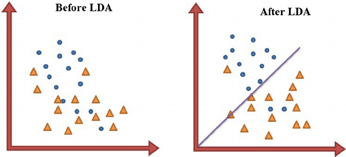
LDA, in contrast to PCA, is a “supervised method”, i.e. that it computes the directions (called “linear discriminants”) that will represent the axes that maximize the separation between multiple classes.
Data sets can be transformed and test vectors can be classified in the transformed space by two different approaches (Balakrishnama, S., Aravind G., 1998)
- Class-dependent transformation: This type of approach involves maximizing the ratio between-class variance to within-class variance. The main objective is to maximize this ratio so that adequate class separability is obtained. The class-specific type approach involves using two optimizing criteria for transforming the data sets independently.
- Class-independent transformation: This approach involves maximizing the ratio of overall variance to within-class variance. This approach uses only one optimizing criterion to transform the data sets and hence all data points irrespective of their class identity are transformed using this transform. In this type of LDA, each class is considered as a separate class against all other classes.
Why do we use linear discriminant analysis?
There are several reasons why we use the LDA for classification tasks instead of logistic regression:
- when the classes are well-separated, the parameter estimates for the
logistic regression model are surprisingly unstable. The linear discriminant analysis does not suffer from this problem. - when there are few examples and the distribution of the predictors X is approximately normal in each of the classes, the linear discriminant model is more stable than the logistic regression model.
- linear discriminant analysis is more popular when we have more than two response classes.
Linear Discriminant Analysis With Python
To demonstrate the implementation of LDA in Python I will use scikit-learn Python machine learning library and the LinearDiscriminantAnalysis class.
For this tutorial I will use the Wine Dataset. This dataset is public available for research purposes only, for more information see: UCI Machine Learning Repository
The dataset isrelated to red and white variants of the “Vinho Verde” wine.
UCI Notes About the Dataset:
- The classes are ordered and not balanced (e.g. there ismunch more normal wines than excellent or poor ones).
- Outlier detection algorithms could be used to detect the few excellent or poor wines.
- Also, we are not sure if all input variables are relevant. So it could be interesting to test feature selection methods.
Note: for simplicity, we are not going to deep dive into data preprocessing.
First, let’s import libraries and read the data.
Next, we need to define the model.
We will fit and evaluate a Linear Discriminant Analysis model using repeated stratified k-fold cross-validation via the RepeatedStratifiedKFold class. We will use 10 folds and three repeats.
In this case, we can see that the model achieved a mean accuracy of about 98.9 percent.
How To Tune LDA Hyperparameters
There are two important hyperparameters for the Linear Discriminant Analysis method you can consider to tune:
solver : string, possible values:
- svd: Singular value decomposition (default).
Does not compute the covariance matrix, therefore this solver is
recommended for data with a large number of features.
- eigen: Eigenvalue decomposition, can be combined with shrinkage.
shrinkage : string or float, possible values:
- None: no shrinkage (default).
- auto: automatic shrinkage using the Ledoit-Wolf lemma.
- float between 0 and 1: fixed shrinkage parameter.
Note: shrinkage works only with ‘lsqr’ and ‘eigen’ solvers.
Shrinkage adds a penalty to the model that acts as a type of regularizer, reducing the complexity of the model.
The example below demonstrates this using the GridSearchCV class with a grid of different solver values.
The code above will evaluate each combination of configurations using repeated cross-validation.
In this case, we can see that the default SVD solver performs the best compared to the other built-in solvers
Now, we will see whether using shrinkage improves model performance.
In this case, we can see that using shrinkage does not have an impact on classification results.
Conclusion
Linear Discriminant Analysis can be used as a tool for classification, dimension reduction, and data visualization. Despite its simplicity, LDA can produce robust, decent, and interpretable classification results.
In this article, I demonstrated how to use Linear Discriminant Analysis for classification machine learning algorithm in Python. Specifically, I described:
- what LDA is,
- why do we use linear discriminant analysis,
- how to implement Linear Discriminant Analysis with Python,
- how to tune LDA hyperparameters.