As during the first two articles, first we need to import the librairies, the data, and define the constants (see other articles for further details):
Once we have imported the data, time is now to create two backtesting functions. The first one is a function that computes the earnings and loss, given a specific set of stoploss, takeprofit and the exchange fees. This step is important so that our backtesting is coherent with real-life trading conditions. In the previous step I defined fees = 0.125%, which corresponds to the Poloniex [2] exchange fees.
The second function really is the backtesting function. It takes the testing set as input, the model which we want to backtest, and our constants. It then compute the predictions over the test set, and computes the backtested earnings in a column named ‘EarningsBullish’. As we seek to build a bullish trading bot, we filter out the bearish predictions (preds = 0).
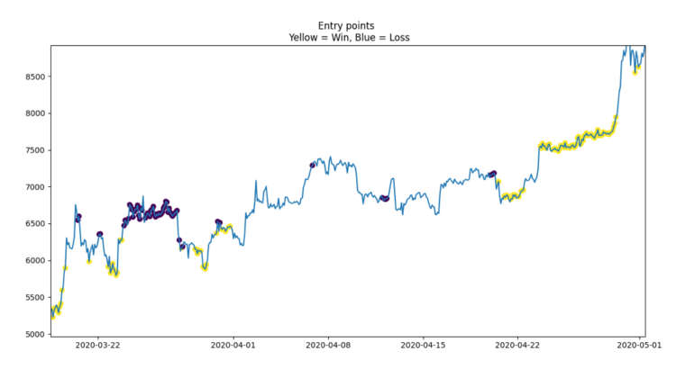
Once we have defined our backtesting functions, we can try to look at a first approach. This approach is simply to follow the best model’s bullish predictions. We then display the PnL (Profits And Loss) profile, the entry points, and the ROI (Return On Investment). Finally, we may wish to evaluate to which degree the performance is great. To do this, we compare the approach’s performance to the average return over the testing period (with stoploss and takeprofit) : that is, we look at the expected returns if we’d always bet bullish at each timestep. With this technique, we can really assess the performance of our method, independently of the market’s conditions. We will obtain a metric called avg_return_benchmark, which we will compare to our performance and test the statistical significance of our performance and the average benchmark through a t-test [3].
The performance is superior to the benchmark, however it is not yet significative (p-value > 0.05).
What we obtain in the case of our example is like this :
The code to generate and backtest this first strategy is the following :
As presented earlier, the principle of this second approach can be summarized as following : we pick the best model, and look for the threshold l such that limiting the trades to cases where proba_bullish > l yields the most profitable strategy. To do this, we need to evaluate the best model on the validation_set, otherwise the approach would not be generalizable. The very first step is to create a function that create a recapitulative table such like this one :
Once we have computed and saved this table, we simply pick the threshold which yields the best ROI. In our example we can see that the best threshold is l =0.85. We can then evaluate this strategy (keeping predictions where proba_best_model > 0.85) on the test set so that we can see how this approach performs on totally new data. We observe that the strategy is once again yielding great profits, with a ROI that is even higher than during the first approach. The performance is now significative (p-value < 0.05), which is a great point :
The code to generate the second approach is written down there :
First we may recall that the full code is available at [4].
During this article, we have created two profitable trading strategies. These strategies perform better than the benchmark — i.e. they are accurate and yield sufficient profit — and the latter is even yielding significant results. We checked that the strategies were yielding profit on totally new data, which lets indicate that their real-life implementation will also generate profits in the long run.
Now that we have identified and backtested our strrategies, we may wish to implement them for real-life trading. That is exactly the purpose of the next article, which will expose how one can create such trading bot in Python. The trading bot will be developed with the Poloniex API, which is a cryptocurrencies exchange platform. However, the framework can easily be adapted to any other API or coding system.
Also, the full paper that I wrote concerning an advanced trading bot is available at [5].
