Python implementation, Attention Mechanism. Additive and Multiplicative attention.
Attention has been a huge area of research. It is widely used in various sub-fields, such as Natural Language Processing or Computer Vision. This article is an introduction to Attention Mechanism that tells about basic concepts and key points of the Attention Mechanism. There are to fundamental methods introduced that are Additive and Multiplicative Attentions, also known as Bahdanau and Luong Attention respectively. For the purpose of simplicity, I take a language translation problem, for example English to German, in order to visualize the concept. Thus, both Encoder and Decoder are based on a Recurrent Neural Network (RNN).
As it can be seen the task was to translate “ Orlando Bloom and Miranda Kerr still love each other” into German. The base case is a prediction that was derived from a model based on only RNNs, whereas the model that uses Attention Mechanism could easily identify key points of the sentence and translate it effectively. If you are new to this area, let’s imagine that the input sentence is “tokenized” breaking down the input sentence into something similar:
[<start>, orlando, bloom, and, miranda, kerr, still, love, each, other, <end>]
Then these tokens are converted into unique indexes each responsible for one specific word in a vocabulary. So, the example above would look similar to:
[ 0, 33, 34, 3, 44, 45, 6, 7, 8, 9, 1]
Attention Encoder
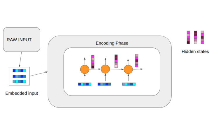
The image above is a high level overview of how our encoding phase goes. In this example the encoder is a Recurrent Neural Network (RNN). As it can be observed a raw input is pre-processed by passing through an embedding process. In real world applications the embedding size is considerably larger; however, the image showcases a very simplified process. So, the colored boxes represent our vectors, where each color represents a certain value. Thus, at each timestep, we feed our embedded vectors as well as a hidden state derived from the previous timestep. Note that for the first timestep the hidden state passed is typically a vector of 0s. Finally, we can pass our hidden states to the decoding phase.
Attention Decoder
As we might have noticed the encoding phase is not really different from the conventional forward pass. However, in this case the decoding part differs vividly. As it can be observed, we get our hidden states, obtained from the encoding phase, and generate a context vector by passing the states through a scoring function, which will be discussed below. Thus, in stead of just passing the hidden state from the previous layer, we also pass a calculated context vector that “manages” decoder’s attention. Note that the decoding vector at each timestep can be different. Also, if it looks confusing the first input we pass is the end token of our input to the encoder, which is typically <end> or <eos>, whereas the output, indicated as red vectors, are the predictions.
This mechanism refers to Dzmitry Bahdanau’s work titled “Neural Machine Translation by Jointly Learning to Align and Translate”. Thus, this technique is also known as Bahdanau Attention. The Additive Attention is implemented as follows
where h_j is j-th hidden state we derive from our encoder, s_i-1 is a hidden state of the previous timestep (i-1th), and W, U and V are all weight matrices that are learnt during the training. Then, we pass the values through softmax which normalizes each value to be within the range of [0,1] and their sum to be exactly 1.0. Thus, we expect this scoring function to give probabilities of how important each hidden state is for the current timestep. Finally, we multiply each encoder’s hidden state with the corresponding score and sum them all up to get our context vector.
Read More: Neural Machine Translation by Jointly Learning to Align and Translate
This method is proposed by Thang Luong in the work titled “Effective Approaches to Attention-based Neural Machine Translation”. It is built on top of Additive Attention (aka Bahdanau Attention). There are three scoring function that we can choose from.
The main difference here is that only top RNN layer’s hidden state is used from the encoding phase, allowing both encoder and decoder to be a stack of RNNs. The first option, which is dot, is basically a dot product of hidden states of the encoder (h_s) and the hidden state of the decoder (h_t). The latter one is built on top of the former one which differs by 1 intermediate operation. Finally, concat looks very similar to Bahdanau attention but as the name suggests it concatenates encoder’s hidden states with the current hidden state.
Finally, in order to calculate our context vector we pass the scores through a softmax, multiply with a corresponding vector and sum them up.
Read More: Effective Approaches to Attention-based Neural Machine Translation
If you are a bit confused a I will provide a very simple visualization of dot scoring function. I hope it will help you get the concept and understand other available options 🙂
Dot scoring:
Suppose our decoder’s current hidden state and encoder’s hidden states look as follows: