In both cases, histogram analysis revealed that in images with low-contrast:
- the pixel intensities are concentrated in a narrow region resulting in pixels with similar shades, giving the image a faded appearance, and
- the cumulative histogram increases with a steep slope within a narrow region and flat elsewhere.
The contrast of an image is enhanced when various shades in the image becomes more distinct. We can do so by darkening the shades of the darker pixels and vice versa. This is equivalent to widening the range of pixel intensities. To have a good contrast, the following histogram characteristics are desirable:
- the pixel intensities are uniformly distributed across the full range of values (each intensity value is equally probable), and
- the cumulative histogram is increasing linearly across the full intensity range.
Histogram equalization modifies the distribution of pixel intensities to achieve these characteristics.
Step 1: Calculate normalized cumulative histogram
First, we calculate the normalized histogram of the image. Normalization is performed by dividing the frequency of each bin by the total number of pixels in the image. As a result, the maximum value of the cumulative histogram is 1. The following figure shows the normalized cumulative histogram of the same low contrast image presented as Case 1 in Section 3.
Step 2: Derive intensity-mapping lookup table
Next, we derive a lookup table which maps the pixel intensities to achieve an equalized histogram characteristics. Recall that the equalized cumulative histogram is linearly increasing across the full range of intensity. For each discrete intensity level i, the mapped pixel value is calculated from the normalized cumulative histogram according to:
mapped_pixel_value(i) = (L-1)*normalized_cumulative_histogram(i)
where L = 256 for a typical 8-bit unsigned integer representation of pixel intensity.
As an intuition into how the mapping works, let’s refer to the normalized cumulative histogram shown in the figure above. The minimum pixel intensity value of 125 is transformed to 0.0. The maximum pixel intensity value of 200 is transformed to 1.0. All the values in between are mapped accordingly between these two values. Once multiplied by the maximum possible intensity value (255), the resulting pixel intensities are now distributed across the full intensity range.
Step 3: Transform pixel intensity of the original image with the lookup table
Once the lookup table is derived, intensity of all pixels in the image are mapped to the new values. The result is an equalized image.
Histogram equalization is available as standard operation in various image processing libraries, such as openCV and Pillow. However, we will implement this operation from scratch. We will need two Python libraries: NumPy for numerical calculation and Pillow for image I/O. The easiest way to install these libraries is via Python package installer pip . Enter the following commands on your terminal and you are set!
pip install numpy
pip install pillow
The full code is show below, followed by detailed explanation of the equalization process. To equalize your own image, simply edit the img_filename and save_filename accordingly. A demo Jupyter notebook and sample image are also available from my github repository.
Image I/O
To read from and write to image files, we will use Pillow library. It reads image files as Imageobject. These objects can be converted easily to NumPy array, and viceversa. The required I/O operations are coded as follows. For simplicity, let the image filename be input_image.jpg residing in the same directory as as the Python script.
import numpy as np
from PIL import Imageimg_filename = 'input_image.jpg'
save_filename = 'output_image.jpg'#load file as pillow Image
img = Image.open(img_filename)# convert to grayscale
imgray = img.convert(mode='L')#convert to NumPy array
img_array = np.asarray(imgray)
#PERFORM HISTOGRAM EQUALIZATION AND ASSIGN OUTPUT TO eq_img_array
#convert NumPy array to pillow Image and write to file
eq_img = Image.fromarray(eq_img_array, mode='L')
eq_img.save(save_filename)
Histogram Equalization
The main algorithm can be implemented in only several lines of code. In this example, the intensity-mapping lookup table is implemented as 1D list where the index represents the original image pixel intensity. The element at each index is the corresponding transformed value. Finally, there are various ways to perform the pixel intensity mapping. I used list comprehension by flattening and reshaping the 2D image array before and after the mapping.
"""
STEP 1: Normalized cumulative histogram
"""#flatten image array and calculate histogram via binning
histogram_array = np.bincount(img_array.flatten(), minlength=256)#normalize
num_pixels = np.sum(histogram_array)
histogram_array = histogram_array/num_pixels#cumulative histogram
chistogram_array = np.cumsum(histogram_array)
"""
STEP 2: Pixel mapping lookup table
"""
transform_map = np.floor(255 * chistogram_array).astype(np.uint8)
"""
STEP 3: Transformation
"""# flatten image array into 1D list
img_list = list(img_array.flatten())# transform pixel values to equalize
eq_img_list = [transform_map[p] for p in img_list]# reshape and write back into img_array
eq_img_array = np.reshape(np.asarray(eq_img_list), img_array.shape)
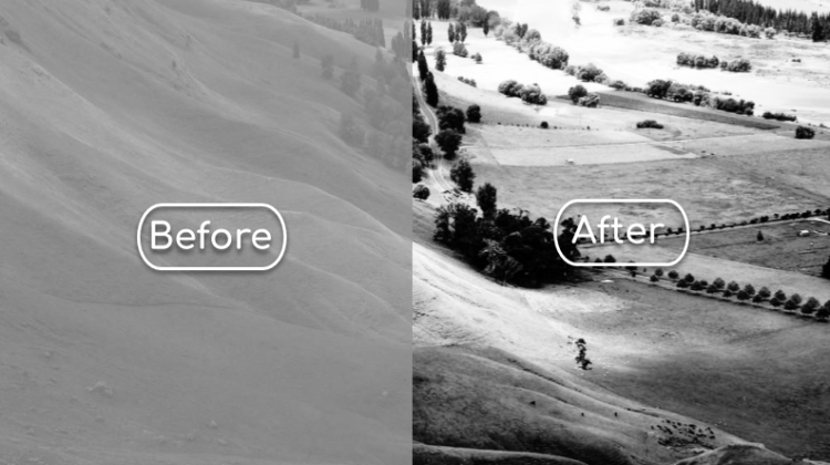
Let’s look at the histogram equalization output for the two images presented in Section 3. For each result, the upper two images show the original and equalized images. Improvement in contrast is clearly observed. The lower two images show the histogram and cumulative histogram, comparing original and equalized images. After histogram equalization, the pixel intensities are distributed across the whole intensity range. The cumulative histograms are increasing linearly as expected, while exhibiting staircase pattern. This is expected as the pixel intensities of the original image were stretched into a wider range. This creates gaps of bins with zero frequency between adjacent non-zero bins, appearing as flat line in the cumulative histogram.