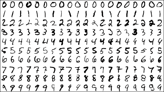
Previously we were learning how to create different parts of neural networks. To train different versions of our artificial intelligence we used abstract training data. And now the time has come to use real data.
Data
We are going to teach our neural net to recognize handwritten digits with help of MNIST dataset. Also known as the “hello world problem” in the machine learning industry.
MNIST dataset contains 60 000 labeled data points (images) as training dataset and 10 000 testing dataset. Original data stored in binaries files so we will need to do some extraction work. You can find the same dataset on Kaggle in more user-friendly form, but we aren’t looking for an easy way out.
The data in the file IDX file is stored as vectors in multidimensional matrices space. To extract data from an IDX file we will need to separate each dimension of the matrix and then each data point, which in our case, will be the pixel. Then we will use numpy method shape data in the form of familiar arrays for us. And library gzip will help us open and read the IDX file. That’s how you do it for the training set:
And that’s how we extract training labels (it’s an one dimensional array that’s why it’s shorter):
And I would save this data into the JSON file so we don’t have to repeat the formatting process every time we need to run the code.
Preprocessing data
We have data available in the python friendly format so we can start working with it. And the next we will do several operations to cook our data so the neural network can digest it.
First step is normalization. We are going to use a min-max normalization method which will convert values of all pixels in range [-1:1]. -1 is a completely white pixel and 1 is black. We need to do that because the original values of the pixels are in [0:255] and neural networks prefer (work faster) to work with values between -1 and 1.
Second step will be reshaping the 2-x dimensional array into the one dimensional. We will need it to make matrices align so it will be possible to extract dot products.
On the third step we will shuffle our data so it’s reducing variance and ensuring that models become more general and not overfit much.
And the final step of the preprocessing is reshape labels dataset. Right now it’s in the form of a 1x dimensional array and each value corresponds with each image from the training dataset. What we need to do is to convert each label into the array size of the output layer (10 in our case) and populate it with 0s. And replace 0 to 1 in the index which matches with the number in the original labels dataset.
Batching
Previously we were working with a pretty simple dataset and it was possible to just feed the whole thing into the neural network. But now we are dealing with a much bigger dataset and if you try to load it all the computer will tell you that you are insane and it doesn’t have that much ram memory to store so much data. The solution is to divide data in batches and feed it one by one. Size of the batch depends on your machine resources and usually within a range between 16 and 128 elements per batch.
This is how we batching out data:
And we will need to modify the learning process a a bit to load one batch at the time:
Training and evaluating
The training process remains pretty much the same as in the last article about neural networks. The only difference is amount of data we going to feed to out network. It’s all the same sigmoids, softmax and derivatives. Check out my previous posts about different parts of the learning process.
And to test how well our model performs after the training we have 10 000 labeled examples to try it out. You will need to extract it from the MNIST dataset the same way we extracted training data, but from different files. Here the testing function I created:
Check out final code:
Conclusion
Finally we get to work with a real world dataset. Only after training my first model on the MNIST dataset I realized why in time the first Rosenblatt perceptron neural networks did not succeed. Because it’s a very expensive computational task. And at that time computational power of my desktop wasn’t available even to the US military researchers.
And this is how our model performed with parameters declared in the code:
Like we can see error rate is only 1.97%, it’s pretty good for the neural network built from scratch. Now we can come up with use cases and create applications which will be powered with Artificial Intelligence!
Keep learning, keep growing!
