Reducing high dimension features to low dimension features
In this article, we will discuss the feature reduction methods that deals with over-fitting problems occurs in large number of features. When a high dimension data fits in the model then it confused sometimes in between features of similar information. To find the main features/components that are going to impact more on target variable and those components have maximum variance. The 2-dimension feature convert to 1- dimension feature so that computational will be fast.
In machine Learning, the dimensions are the number of features in the data set. As the more dimension added in the data then it will make more dimension space exponentially with this it will cost more for processing that cause “curse of dimensionality”.
Why reduce the dimensions?
- We know that for training large dimension data need more computation power and time.
- Visualization is not possible with large dimensional data.
- More dimensions means more storage space problem.
Two techniques with which we can reduce the dimensions as shown below:
- Feature Selection: These are backward elimination, forward selection and bidirectional elimination.
- Feature Extraction: These are principal component analysis(PCA), Linear discriminant analysis (LDA), kernel PCA and others.
The PCA reduce the n feature to n≤p components features that explain the most the variance of the dataset.
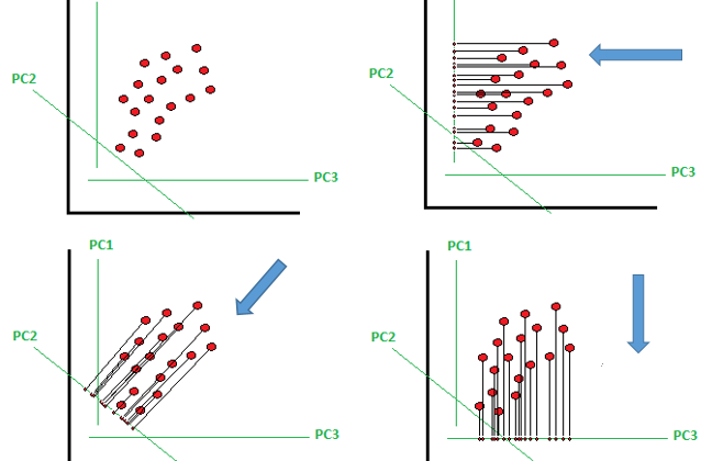
Principal components are linear combination (orthogonal transformation) of the original predictor in the data set.
If there are many principal components then the first PC1 have the maximum variance and later PC2, PC3,…. variance decrease. The PC1 and PC2 have a zero correlation.
The processing limitation in PCA is that it takes all the data in the memory in one batch. So, need of large memory, to avoid this one time memory use there is a incremental PCA comes into role that process uses mini batch processing that almost matches the result as with PCA.
Example with python:
Importing the necessary libraries
import numpy as np
import pandas as pd
Reading the dataset from url
url = "https://archive.ics.uci.edu/ml/machine-learning-databases
/iris/iris.data"names=['sepal-length','sepal-width','petal-length','petal-
width','Class']df = pd.read_csv(url,names=names)
To view the first 5 rows with head method.
df.head()
Divide the data into independent and dependent features.
X=df.drop('Class',1)
y = df['Class']
Now, divide the features in train and test set.
from sklearn.model_selection import train_test_split
X_train, X_test, y_train, y_test = train_test_split(X,y,test_size = 0.2)
Using the standard scalar to standardize the data set values.
from sklearn.preprocessing import StandardScaler
sc = StandardScaler()
X_train = sc.fit_transform(X_train)
X_test = sc.transform(X_test)
Now, here is our player of this article, using PCA from decomposition class.
#Apply PCA
from sklearn.decomposition import PCA
pca = PCA()
X_train = pca.fit_transform(X_train)
X_test = pca.transform(X_test)
After this we have to know the variance of all principal components
explained_variance = pca.explained_variance_ratio_
print(explained_variance)#output:
array([0.71580568, 0.24213308, 0.03690989, 0.00515135])
We can use n_components parameter to use the number of principal components.
#Try out with only 1 PCA
#Apply PCA
from sklearn.decomposition import PCA
pca = PCA(n_components=1)
X_train = pca.fit_transform(X_train)
X_test = pca.transform(X_test)
Now we can use these x_train and x_test values in our algorithm.
from sklearn.ensemble import RandomForestClassifier
classifier = RandomForestClassifier()
classifier.fit(X_train,y_train)#output:RandomForestClassifier(bootstrap=True, class_weight=None,
criterion='gini', max_depth=None, max_features='auto',
max_leaf_nodes=None, min_impurity_decrease=0.0,
min_impurity_split=None, min_samples_leaf=1,
min_samples_split=2, min_weight_fraction_leaf=0.0,
n_estimators=10, n_jobs=None,oob_score=False,
random_state=None, verbose=0, warm_start=False)
Now, we will predict out model and will check the accuracy.
y_pred = classifier.predict(X_test)
from sklearn.metrics import accuracy_score
print('Accuracy of this model is' , accuracy_score(y_test,y_pred))#output:
Accuracy of this model is 0.9333333333333333
Conclusion:
The PCA works perfectly well with high dimension data. The richness of PCA is it reduces the training cost time.
I hope you like the article. Reach me on my LinkedIn and twitter.
2. Python Data Structures Data-types and Objects
3. Python: Zero to Hero with Examples
4. Fully Explained SVM Classification with Python
5. Fully Explained K-means Clustering with Python
6. Fully Explained Linear Regression with Python
7. Fully Explained Logistic Regression with Python
8. Basics of Time Series with Python