Chapter 2
Last time in Chapter 1 we discussed, what is Machine Learning and what are its types if you haven’t read about it I would recommend you to go through the previous article. Okay, so moving forward today we’ll discuss some more concepts.
Let’s start.
So before starting, I would like to throw some light on what is a machine learning model. A machine learning model is a file or a program that is trained with data sets so it could figure out some kind of pattern or relationship between given data. And after the model is trained then it is fed with some data unknown to it and then the model is expected to provide an output based on its logic or pattern it observed while training.
For Example, Let’s say you want to have an application that recognizes fruits. So you will train your model with a humongous size labelled dataset(collection of samples that are already tagged/labelled for training models) and then you can use that model in an application that can recognize any fruit.
So, the definition of Linear regression is as follows:
“Linear regression is a linear model, e.g. a model that assumes a linear relationship between the input variables (x) and the single output variable (y). More specifically, (y) can be calculated from a linear combination of the input variables (x).”
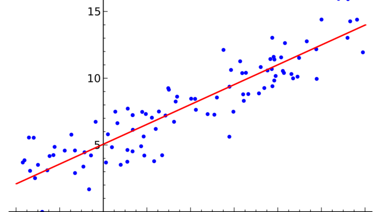
In statistics, Linear regression is a linear approach to form the relationship between a scalar response(dependent variable)and one or more explanatory variables(independent variables).
Mathematically it can be represented as E[Y] = β₀+ β₁X
The case of one explanatory variable is also known as simple linear regression and when there are multiple input variables, literature from statistics often refers to the method as multiple linear regression.
One must ask why to use linear regression answer is because of its easy representation. In Linear regression, the relationship is modelled using a linear predictor function whose unknown model parameters are estimated from data. This type of model is known as the Linear Model.
The hypothesis of Linear Regression
The linear regression model can be represented by the following equation
- Y is the predicted value
- θ₀ is the bias term.
- θ₁,…,θₙ are the model parameters
- x₁, x₂,…,xₙ are the feature values.
The above hypothesis can also be represented by
where
- θ is the model’s parameter vector including the bias term θ₀
- x is the feature vector with x₀ =1
Assumptions in Linear Regression
There are certain assumptions made in linear regression which are as follows:
- Linearity: It is considered that the relation between X and the mean of Y should always be linear.
- Homoscedasticity: In statistics, homoscedasticity means homogeneity invariance. So in linear regression, we consider that variance of residual is the same for any value of X.
- Independence: It is considered that no observation is correlated, every observation is independent in itself.
- Normality: For any fixed value of X and Y is normally distributed.
Cost Function
This function is basically used for measuring the accuracy of our hypothesis function(discussed in Chapter 1) so we can get a best-fit line. So when we are finally using our prediction model, it will predict the value of Y for the input value of X. So, it is very important to update the θ₁ and θ₂ values, to reach the best value that minimizes the error between the predicted Y value (predᵢ) and true Y value (Yᵢ).
Mathematically,
This function is also known as “Squared Error Function” or “Mean Squared Error”.
The mean is halved(½) as a convenience for computation of gradient descent, as the derivative term of the square function will cancel out the (½) term.
So idea is to choose θ₁ and θ₂ such that the value of ‘predᵢ’ is as close to ‘Yᵢ’ as possible.
What is the Gradient?
“A Gradient is a measure of how much the output changes if we change the input by little” — Lex Fridman. In simpler words, it’s an observation of deviation in output when input is altered.
Gradient Descent is an optimization algorithm for finding a local minimum of a differentiable function. Gradient Descent is simply used to find the values of the function’s parameters(coefficients) that minimizes the cost of the function as much as possible.
Mathematically,
Here ‘α’ is known as the learning rate. So if ‘α’ is large then the learning step is large and vice versa.
To update θ₁ and θ₂ values to reduce the Cost function (minimizing RMSE value) and achieving the best fit line the model uses Gradient Descent. The idea is to start with random θ1 and θ2 values and then iteratively updating the values, reaching minimum cost.
