Last week we talked about Random Forest(RF). We know RF can be used both for regression and classification tasks. This week we will implement the RF on a real-world regression problem.
Our goal here is predict the gasoline consumption in USA, based on values; petrol tax, average income, pawed highways and driver population.
We will use this petrol consumption data-set on kaggle. It’s under CC0 license and free to use.
As I mentioned we will use RF Algorithm via Sci-Kit Learn Python with traditional Machine Learning pipeline.
1- Import the modules
We need to import necessary modules that we will use in this project
#Install the modules if they not exitpip install numpypip install pandaspip install sklearn#Import the modulesimport pandas as pdimport numpy as np
2- Import the Data-Set
We have import our modules and we are ready to work. Lets dive into our data-set.
dataset = pd.read_csv(‘YOUR_DATASET_LOCATION’)
You need to pass your data-set location to the read_csv function. For me it’s look like this:
dataset = pd.read_csv(‘/home/levent/DataSet/petrol_consumption.csv’)
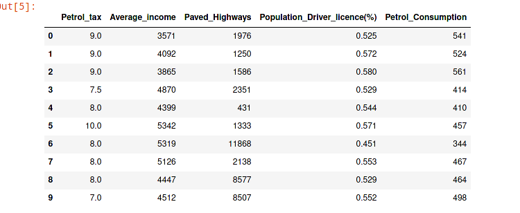
Okay, we have implement our data-set. Now lets run the head function that pandas provides so we can have better observation on our data. Let’s look first 10 rows.
dataset.head(10)
As you see our values are not scaled well. We will scale them before the train the algorithm.
3- Preparing Data For Training
In this section we need tho perform 2 tasks. Firstly, we will divide data into attributes and labels sets. Then we will divide the result to train and test sets.
Lets divide into attributes and labels, we will use pandas iloc for integer-location based indexing for selection by position:
X = dataset.iloc[:, 0:4].values
y = dataset.iloc[:, 4].values
Now lets divide into train and test sets:
from sklearn.model_selection import train_test_splitX_train, X_test, y_train, y_test = train_test_split(X, y, test_size=0.2, random_state=0)
4- Feature Scaling
As you know our data set is not scaled value yet. For this we will use Sci-Kit Learn’s StandartScaler calss. This class will standardize features by removing the mean and scaling to unit variance.
from sklearn.preprocessing import StandardScalersc = StandardScaler()
X_train = sc.fit_transform(X_train)
X_test = sc.transform(X_test)
5- Training the Algorith
Finally we have scale our data. Now it’s time to training the RF algorithm:
from sklearn.ensemble import RandomForestRegressorregressor = RandomForestRegressor(n_estimators=20, random_state=0)
regressor.fit(X_train, y_train)
y_pred = regressor.predict(X_test)
The RandomForestRegressor class from sklearn.ensemble library is used for generate random forest for regression problems. the n_estimators parameter is number of the trees in the forest. We set it 20 for this project. You can have more information about this class here.
6- Evaluating the Algorithm
The final step we need to evaluate the performance our algorithm. For regression problems the metrics used to evaluate an algorithm are mean absolute error, mean squared error, and root mean squared error.
from sklearn import metricsprint('Mean Absolute Error:', metrics.mean_absolute_error(y_test, y_pred))
print('Mean Squared Error:', metrics.mean_squared_error(y_test, y_pred))
print('Root Mean Squared Error:', np.sqrt(metrics.mean_squared_error(y_test, y_pred)))
Output:
Mean Absolute Error: 51.76500000000001
Mean Squared Error: 4216.166749999999
Root Mean Squared Error: 64.93201637097064
With 20 trees, the mean square error is 64.93, which is more than 10 percent of the average gasoline consumption, i.e. 576.77. This may indicate, among other things, that we have not used a sufficient number of estimators (trees).
If the number of estimators is changed to 2000, the results are as follows:
Mean Absolute Error: 48.683
Mean Squared Error: 3533.5014668999997
Root Mean Squared Error: 59.44326258626792
You can play around with the number of trees and other parameters to see if you can get better results on your own.
In the part #3 we will use random forest for real world classification problem.