How to use, implement, and evaluate support vector machines (SVM) in TensorFlow
The following areas will be covered:
- Introduction
- Working with a Linear SVM
Support vector machines are a method of binary classification. The basic idea is to find a linear separating line (or hyperplane) between the two classes. We first assume that the binary class targets are -1 or 1 , instead of the prior 0 or 1 targets. Since there may be many lines that separate two classes, we define the best linear separator that maximizes the distance between both classes.
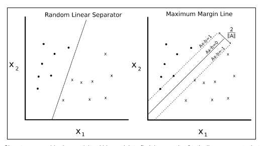
Figure 1: Given two separable classes, ‘o’ and ‘x’, we wish to find the equation for the linear separator between the two. The left shows that there are many lines that separate the two classes. The right shows the unique maximum margin line. The margin width is given by 2/. This line is found by minimizing the L2 norm of A.
We can write such a hyperplane as follows:
Ax-b = 0
Here, A is a vector of our partial slopes and x is a vector of inputs. The width of the maximum margin can be shown to be two divided by the L2 norm of A. There are many proofs out there of this fact, but for a geometric idea, solving the perpendicular distance from a 2D point to a line may provide motivation for moving forward.
For linearly separable binary class data, to maximize the margin, we minimize the L2 norm of A,||A||. We must also subject this minimum to the constraint:
The preceding constraint assures us that all the points from the corresponding classes are on the same side of the separating line
Since not all datasets are linearly separable, we can introduce a loss function for points that cross the margin lines. For n data points, we introduce what is called the soft margin loss function, as follows:
Note that the product yi(Axi-b) is always greater than 1 if the point is on the correct side of the margin. This makes the left term of the loss function equal to zero, and the only influence on the loss function is the size of the margin.
The preceding loss function will seek a linearly separable line, but will allow for points crossing the margin line. This can be a hard or soft allowance, depending on the value of α. Larger values of α result in more emphasis on widening the margin, and smaller values of α result in the model acting more like a hard margin, while allowing data points to cross the margin, if need be.
We will set up a soft margin SVM and show how to extend it to nonlinear cases and multiple classes.
For this example, we will create a linear separator from the iris data set. We know from prior chapters that the sepal length and petal width create a linear separable binary data set for predicting if a flower is I. setosa or not.
To implement a soft separable SVM in TensorFlow, we will implement the specific loss function, as follows:
Here, A is the vector of partial slopes, b is the intercept,xi is a vector of inputs, yi is the actual class (-1,1) and α is the soft separability regularization parameter.
How to do it…
- We start by loading the necessary libraries. This will include the scikit learn dataset library for access to the iris data set. Use the following code:
import matplotlib.pyplot as plt
import numpy as np
import tensorflow as tf
from sklearn import datasets
2. Next we start a graph session and load the data as we need it. Remember that we are loading the first and fourth variables in the iris dataset as they are the sepal length and sepal width. We are loading the target variable, which will take on the value 1 for I. setosa and -1 otherwise. Use the following code:
sess = tf.Session()
iris = datasets.load_iris()x_vals = np.array([[x[0], x[3]] for x in iris.data])
y_vals = np.array([1 if y==0 else -1 for y in iris.target])
3. We should now split the dataset into train and test sets. We will evaluate the accuracy on both the training and test sets. Since we know this data set is linearly separable, we should expect to get one hundred percent accuracy on both sets. Use the following code:
train_indices = np.random.choice(len(x_vals), round(len(x_
vals)*0.8), replace=False)
test_indices = np.array(list(set(range(len(x_vals))) - set(train_
indices)))x_vals_train = x_vals[train_indices]
x_vals_test = x_vals[test_indices]
y_vals_train = y_vals[train_indices]
y_vals_test = y_vals[test_indices]
4. Next we set our batch size, placeholders, and model variables. It is important to mention that with this SVM algorithm, we want very large batch sizes to help with convergence. We can imagine that with very small batch sizes, the maximum margin line would jump around slightly. Ideally, we would also slowly decrease the learning rate as well, but this will suffice for now. Also, the A variable will take on the shape 2×1 because we have two predictor variables, sepal length and pedal width. Use the following code:
batch_size = 100x_data = tf.placeholder(shape=[None, 2], dtype=tf.float32)
y_target = tf.placeholder(shape=[None, 1], dtype=tf.float32)A = tf.Variable(tf.random_normal(shape=[2,1]))
b = tf.Variable(tf.random_normal(shape=[1,1]))
5. We now declare our model output. For correctly classified points, this will return numbers that are greater than or equal to 1 if the target is I. setosa and less than or equal to -1 otherwise. Use the following code:
model_output = tf.sub(tf.matmul(x_data, A), b)
6. Next we will put together and declare the necessary components for the maximum margin loss. First, we will declare a function that will calculate the L2 norm of a vector. Then we add the margin parameter,α. We then declare our classification loss and add together the two terms. Use the following code:
l2_norm = tf.reduce_sum(tf.square(A))alpha = tf.constant([0.1])classification_term = tf.reduce_mean(tf.maximum(0., tf.sub(1., tf.mul(model_output, y_target))))loss = tf.add(classification _term, tf.mul(alpha, l2_norm))
7. Now we declare our prediction and accuracy functions so that we can evaluate the accuracy on both the training and test sets, as follows;
prediction = tf.sign(model_output)
accuracy = tf.reduce_mean(tf.cast(tf.equal(prediction, y_target),
tf.float32))
8. Here we will declare our optimizer function and initialize our model variables, as follows:
my_opt = tf.train.GradientDescentOptimizer(0.01)
train_step = my_opt.minimize(loss)init = tf.initialize_all_variables()
sess.run(init)
9. We now can start our training loop, keeping in mind that we want to record our loss and training accuracy on both the training and test set, as follows:
loss_vec = []
train_accuracy = []
test_accuracy = []for i in range(500):
rand_index = np.random.choice(len(x_vals_train), size=batch_size)
rand_x = x_vals_train[rand_index]
rand_y = np.transpose([y_vals_train[rand_index]])
sess.run(train_step, feed_dict={x_data: rand_x, y_target:rand_y})temp_loss = sess.run(loss, feed_dict={x_data: rand_x, y_target: rand_y})
train_acc_temp = sess.run(accuracy, feed_dict={x_data: x_vals_train, y_target: np.transpose([y_vals_train])})
loss_vec.append(temp_loss)
train_accuracy.append(train_acc_temp) test_acc_temp = sess.run(accuracy, feed_dict={x_data: x_vals_test, y_target: np.transpose([y_vals_test])})
test_accuracy.append(test_acc_temp)if (i+1)%100==0:
print('Step #' + str(i+1) + ' A = ' + str(sess.run(A)) + '
b = ' + str(sess.run(b)))
print('Loss = ' + str(temp_loss))
10. The output of the script during training should look like the following.
Step #100 A = [[-0.10763293]
[-0.65735245]] b = [[-0.68752676]]
Loss = [ 0.48756418]
Step #200 A = [[-0.0650763 ]
[-0.89443302]] b = [[-0.73912662]]
Loss = [ 0.38910741]
Step #300 A = [[-0.02090022]
[-1.12334013]] b = [[-0.79332656]]
Loss = [ 0.28621092]
Step #400 A = [[ 0.03189624]
[-1.34912157]] b = [[-0.8507266]]
Loss = [ 0.22397576]
Step #500 A = [[ 0.05958777]
[-1.55989814]] b = [[-0.9000265]]
Loss = [ 0.20492229]
11.In order to plot the outputs, we have to extract the coefficients and separate the x values into I. setosa and non- I. setosa, as follows:
[[a1], [a2]] = sess.run(A)
[[b]] = sess.run(b)
slope = -a2/a1y_intercept = b/a1
x1_vals = [d[1] for d in x_vals]
best_fit = []for i in x1_vals:
best_fit.append(slope*i+y_intercept)setosa_x = [d[1] for i,d in enumerate(x_vals) if y_vals[i]==1]
setosa_y = [d[0] for i,d in enumerate(x_vals) if y_vals[i]==1]
not_setosa_x = [d[1] for i,d in enumerate(x_vals) if y_vals[i]==-1]
not_setosa_y = [d[0] for i,d in enumerate(x_vals) if y_vals[i]==-1]
12. The following is the code to plot the data with the linear separator, accuracies, and loss:
plt.plot(setosa_x, setosa_y, 'o', label='I. setosa')
plt.plot(not_setosa_x, not_setosa_y, 'x', label='Non-setosa')
plt.plot(x1_vals, best_fit, 'r-', label='Linear Separator', linewidth=3)
plt.ylim([0, 10])
plt.legend(loc='lower right')
plt.title('Sepal Length vs Pedal Width')
plt.xlabel('Pedal Width')
plt.ylabel('Sepal Length')
plt.show()
Using TensorFlow in this manner to implement the SVD algorithm may result in slightly different outcomes each run. The reasons for this include the random train/test set splitting and the selection of different batches of points on each training batch. Also, it would be ideal to also slowly lower the learning
rate after each generation.
Final linear SVM fit with the two classes plotted:
plt.plot(train_accuracy, 'k-', label='Training Accuracy')
plt.plot(test_accuracy, 'r--', label='Test Accuracy')
plt.title('Train and Test Set Accuracies')
plt.xlabel('Generation')
plt.ylabel('Accuracy')
plt.legend(loc='lower right')
plt.show()
because the two classes are linearly separable.
Test and train set accuracy over iterations. We do get 100% accuracy because the two classes are linearly separable:
plt.plot(loss_vec, 'k-')
plt.title('Loss per Generation')
plt.xlabel('Generation')
plt.ylabel('Loss')
plt.show()
How it works…
we have shown that implementing a linear SVD model is possible by using the
maximum margin loss function.
Logistic regression tries to find any separating line that maximizes the distance (probabilistically), SVMs also try to minimize the error while maximizing the margin between classes. In general, if the problem has a large number of features compared to training examples, try logistic regression or a linear SVM. If the number of training examples is larger, or the data is not linearly separable, a SVM with a Gaussian kernel may be used.