In today’s article we are going to explore the word vectors. In natural language processing we represent each word as a vector of numbers. These numbers are learnt using various machine learning techniques.
Predicting the countries from the capitals is the problem of finding the analogies. We can write a program that helps us guess the countries from the capitals.
First, as always we have to load the dataset and explore the data.
import pickle
import numpy as np
import pandas as pd
import matplotlib.pyplot as pltfrom utils import get_vectorsdata = pd.read_csv('capitals.txt', delimiter=' ')
data.columns = ['city1', 'country1', 'city2', 'country2']# print first five elements in the DataFrame
data.head(5)
Now we have to predict the relationship between the words. The function we have to write will take three words as input, two of them are related to one another. The function will predict the fourth word which will be related to the third word which is related in the simmilar way as the two previous words.
An example:
Athens is to Greece as Bangkok is to __
First of all, let’s deal with the cosine simmilarity.
𝐴 and 𝐵 represent the word vectors and 𝐴𝑖 or 𝐵𝑖 represent index i of that vector. If they’re completely opposite A = -B then 𝑐𝑜𝑠(𝜃)=−1. If the 𝑐𝑜𝑠(𝜃)=0 then it means that they’re orthogonal. Numbers between 0 and 1 idicate the simmilar score. Numbers between -1 and 0 idicate dissimiar score.
def cosine_similarity(A, B):dot = np.dot(A, B)
norma = np.sqrt(np.dot(A, A))
normb = np.sqrt(np.dot(B, B))
cos = dot/(norma*normb)
return cos
We learn euclidean distance at school. It is the equation to count the distance between two points.
The more similar the words, the more likely the Euclidean distance will be close to 0.
def euclidean(A, B):# euclidean distanced = np.linalg.norm(A-B)return d
Now, when we have written our functions we can use them to find the country for the capital. As previously mentioned we are going to write a function which takes tree words and the embedding dictionary.
def get_country(city1, country1, city2, embeddings):# store the city1, country 1, and city 2 in a set called group
group = set((city1, country1, city2))# get embeddings of city 1
city1_emb = word_embeddings[city1]# get embedding of country 1
country1_emb = word_embeddings[country1]# get embedding of city 2
city2_emb = word_embeddings[city2]# get embedding of country 2 (it's a combination of the embeddings of country 1, city 1 and city 2)
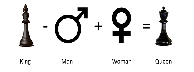
# Remember: King - Man + Woman = Queen
vec = country1_emb - city1_emb + city2_emb# Initialize the similarity to -1 (it will be replaced by a similarities that are closer to +1)
similarity = -1# initialize country to an empty string
country = ''# loop through all words in the embeddings dictionary
for word in embeddings.keys():# first check that the word is not already in the 'group'
if word not in group:# get the word embedding
word_emb = word_embeddings[word]# calculate cosine similarity between embedding of country 2 and the word in the embeddings dictionary
cur_similarity = cosine_similarity(vec,word_emb)# if the cosine similarity is more similar than the previously best similarity...
if cur_similarity > similarity:# update the similarity to the new, better similarity
similarity = cur_similarity# store the country as a tuple, which contains the word and the similarity
country = (word, similarity)return country
Now we have to test the accuracy of the model.
To measure the accuracy we have to iterate over every row of the dataset and feed them into get_country function.
def get_accuracy(word_embeddings, data):# initialize num correct to zero
# loop through the rows of the dataframe
num_correct = 0
for i, row in data.iterrows():# get city1
city1 = row['city1']# get country1
country1 = row['country1']# get city2
city2 = row['city2']# get country2
country2 = row['country2']# use get_country to find the predicted country2
predicted_country2, _ = get_country(city1,country1,city2,word_embeddings)# if the predicted country2 is the same as the actual country2...
if predicted_country2 == country2:
# increment the number of correct by 1
num_correct += 1# get the number of rows in the data dataframe (length of dataframe)
m = len(data)# calculate the accuracy by dividing the number correct by m
accuracy = num_correct/m
return accuracy
PCA allows to reduce the dimensions of the word vectors. Thanks to that we can easily explore the distance between the vectors because we don’t have to deal with the 300 dimensions. Who can work in 300 dimensions?
You can imagine PCA as method which squeezes the dimensions but still retains the maximum information about the original vectors. In this case by maximum information we mean that the Euclidean distance between the original vectors and their projected siblings is minimal. So the vectors which were close to one another in higher dimensions will be still close to one another.
The steps to compute PCA are as follows:
- Mean normalize the data
- Compute the covariance matrix of your data (Σ)
- Compute the eigenvectors and the eigenvalues of your covariance matrix
- Multiply the first K eigenvectors by your normalized data.
def compute_pca(X, n_components=2):
# mean center the data
X_demeaned = X - np.mean(X,axis=0)# calculate the covariance matrix
covariance_matrix = np.cov(X_demeaned, rowvar=False)# calculate eigenvectors & eigenvalues of the covariance matrix
eigen_vals, eigen_vecs = np.linalg.eigh(covariance_matrix, UPLO='L')# sort eigenvalue in increasing order (get the indices from the sort)
idx_sorted = np.argsort(eigen_vals)# reverse the order so that it's from highest to lowest.
# sort the eigen values by idx_sorted_decreasing
idx_sorted_decreasing = idx_sorted[::-1]
eigen_vals_sorted = eigen_vals[idx_sorted_decreasing]# sort eigenvectors using the idx_sorted_decreasing indices
eigen_vecs_sorted = eigen_vecs[:,idx_sorted_decreasing]# select the first n eigenvectors (n is desired dimension
# of rescaled data array, or dims_rescaled_data)
eigen_vecs_subset = eigen_vecs_sorted[:,0:n_components]# transform the data by multiplying the transpose of the eigenvectors
# with the transpose of the de-meaned data
# Then take the transpose of that product.
X_reduced = np.dot(eigen_vecs_subset.transpose(),X_demeaned.transpose()).transpose()return X_reduced
When we plot the words we can notice that words with the simmilar meaning like happy or sad are close to one another.
