In the last two articles, we saw a number of methods to independently estimate AR(p) and MA(q) coefficients, namely the Yule-Walker method, Burg’s Algorithm, and the Innovations Algorithm, as well as the Hannan-Risennan Algorithm, to jointly estimate ARMA(p,q) coefficients, by making use of initialized AR(p) and MA(q) coefficients with the previous algorithms. We also mentioned, that these methods, as sophisticated as they are, tend to perform quite poorly when it comes to dealing with real datasets, as it’s easy to misspecify the true model. Therefore, we would like to yer introduce another assumption: normality of the observations. These are called Gaussian Time Series.
Gaussian Time Series
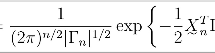
Then its likelihood follows a multivariate normal density given by
where
Note that Gamma_{n} is indeed a function of the parameters that we are trying to maximize (that’s it, the phi’s for the AR(p) part, the thetas for the MA(q), and the sigma squared for the common variance). This follows as K(i,j) is indeed a function of the autocovariance function, which in turn contains such parameters, depending on the actual model. Therefore, we would like to be able to maximize this likelihood to obtain the most suitable set of parameters of the model. However, the presence of the Gamma_n matrix presents two huge problems: calculations and maximizations of its inverse and determinant are extremely computationally costly and do not provide a “friendly” gradient either.
Innovations Algorithm for Gaussian Time Series
So, how can we actually solve this issue? Once again, the Innovations Algorithm comes to the rescue. By considering the Innovations instead of the actual observations by themselves, we can express the previous likelihood as
where
are functions of the phi and theta parameters, but not of sigma squared.
Proof
be the coefficients from the Innovations Algorithm.
is the prediction error for the j-th observation.
- Recall the matrix C_{n}, defined as
- Recall as well that form the Innovations algorithm, we also have that
, that is, Innovations are uncorrelated, which implies that
- This further implies that the vector of innovations
has a diagonal covariance matrix, given by
where the diagonal entries come directly from the Innovations algorithm, since
That is, these are given by the recursive formula
Using these facts, we have that
, from which follows that
That is, we can replace in the likelihood:
For the determinant, we have that
So that we can then write down the likelihood as
But wait! Although we have indeed achieved to express the likelihood in a rather nice form, we still cannot optimize for the sigma square parameter independently. Recall that for the ARMA(p,q), the Innovations algorithm defines W_{t} as
, from which it follows that
, so that
Therefore, we can conclude that
Note: Recall that for the ARMA(p,q) model, K{i,j} is given by
, from which you can more clearly see the dependence on the parameters. See my article on Innovations Algorithm for ARMA(p,q) models.
Gaussian MLE estimates of ARMA(p,q) model
Now the question is: how do we optimize such likelihood? It turns out that we can find MLE estimates of the form
and,
Proof
We can perform some simple algebraic manipulation as follows. First, we apply the natural logarithm to the likelihood, obtaining
Solving w.r.t. sigma square yields the respective estimate. Now, plugging this back into the likelihood yields:
Ignoring the constants, this implies that the MLE estimates of the phi and theta parameters are given by
Note
- Consider the SS_{Res} (Sum of Squared Residuals)
Inside the summation, the numerator is the square prediction error given by the squared difference between each observation and its estimate given by the suitable BLP under some parameters phi’s and theta’s. This is then normalized by the MSE of that prediction.
- What makes an innovation “unlikely”?
Note that
Therefore, we see that this natural normalization is necessary because simply considering the innovations would give too much weight to early observations. By normalizing, they are on “equal footing”.
the second term can be seen as a kind of geometric mean regularization, giving an extra penalty on the likelihood for large values of r_{j}.
- Note that the optimization problem above has no closed-form solution. However, we can use numerical optimization algorithms such as gradient descent or Newton-Raphson. These algorithms, however, require initial values for the parameters in question; therefore choosing “good starting values” can yield better estimates and ensure faster convergence. Some good options are estimates produced by other algorithms, such as Burg’s algorithm and Hannan-Rissanen’s.
- Before modern optimization methods, people used to perform lazy optimization, in which the optimization objective was simplified to
This way, it can be solved analytically, producing the estimates
However, these estimates often produce non-causal and/or non-invertible solutions, without placing additional constraints, which would yield once again a similar objective to the one we originally presented.
Asymptotic Normality of Gaussian MLE Estimates
Now let’s just see a couple of normality properties of the resultant coefficients. These are useful in obtaining things like confidence intervals for the parameter values, for instance. Let
be the true parameters from the MLE estimates in the previous section. Then, for large n
where
for
for
In practice, we can approximate the variance matrix by the hessian of the parameters, given by
where
This is convenient because the Hessian is usually calculated as a part of some optimization algorithms.
Last time
Estimation of ARMA(p,q) Coefficients (Part II)
Next Time
That’s it! Next time, we will learn about Model Selection for ARMA(p,q) models, and finally see some comprehensive examples on applied time series analysis with ARMA(p,q) models in R. Stay tuned, and happy learning!
Main page
Follow me at
- https://blog.jairparraml.com/
- https://www.linkedin.com/in/hair-parra-526ba19b/
- https://github.com/JairParra
- https://medium.com/@hair.parra