Trying to predict the price of a house based on square feet is a linear regression problem. If you are provided a dataset of known prices of other houses and their respective square feet then we can work out the relationship between them. That is because we know the two quantifiable values of our dataset. From these we can build a linear regression model that shows the relationship between the two variables. If you know the x variable then you will also know the y variable. What if we know our two variables but one is not quantifiable? Lets say we know the Vitamin C content of different types of fruit. Could we predict an apple vs orange based on just the this Vitamin C amount?
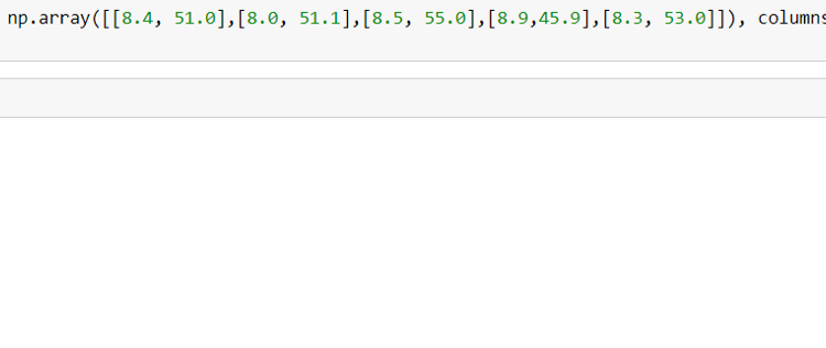
We can create some dummy data with apple and orange vitamin C content and look at a pair plot with a linear regression line.
But this gives us some less than idea results for example lets graph this.
We have some clear relationship where oranges have more Vit-C than apples but what do these points mean? an apple with 8.5 mg of C will correspond to an orange with about 51 mg?
How can we build something similar to this linear regression model if one variable is not a number? As you probably know computers only really understand 1s and 0s. Everything else has just been compiled into combinations of these 1s and 0s. We can use this principle to work with our problem. We can assign the fruit orange to 1 and an apple to 0. Now we have a classification system in place and can create a model to predict 0 or 1 based on Vitamin -C amount.
Lets rebuild this DataFrame with a fruit column giving the glucose content and either a 0or a 1 indicating either apple or orange.
As you can see from above a 0 indicates an apple and a 1 is an orange. Pure linear regression is doing a fairly decent job and you could even say that with fruit glucose readings of below 10 mg of glucose on the x axis looks like would indicate an an apple and round to 0. Conversely above about 40 mg maps to about .80 on the index and we would round to 1 placing it in the orange category. However if you look in our training data we see our oranges and apples and are line is never correct. It’s not telling us where the oranges and apples are and just sits between them. Moreover with this dataset we do not have any outliers. Even one outlier of maybe a really low sugar apple or a really extremely sweet orange would make this linear regression model move almost horizontal. This limits the models predicable capabilities and thus useless.
As you can tell our single outlier moved the model significantly and now even a glucose reading of 60 mg would not properly capture the oranges.
To solve this mathematicians use what is called logistic regression as our modeling technique for classification problems. The sigmoid function also known as the logistic regression function:
This sigmoid function will always between 1 and 0. and as you can see it is a much better fit for our example where apples were either 0 and oranges were 1. Logistic Regression aims to show a probability of what we can think of as on or off, 0 or 1, true or false.
log_loss_function = -ylog(ŷ)-(1-y)log(1-ŷ)
Logistic Regression aims to minimize the Log Loss equation where ŷ is the average of the sum of the predicted y values and y is the actual y values. Much like Linear Regression where we minimize the vertical distances between the data points and the regression line.
If y = 1 then the second part of the equation cancels out and our function is the negative of log(ŷ)
if y=1 log_loss = -log(ŷ)
However if y=0
y=0 log_loss = -log(1-ŷ)
This log loss equation will produce 0 for correctly classified points giving us the low value we want. However bad classifications will give us large numbers and hurt the minimization process.
Before we go further we need to discuss how we can gauge how good our model is. To do so Machine Learners utilize what is known as a Confusion Matrix. This grid has two columns and two rows both of which show True vs Predicted Values.
The best part of Logistic Regression is it will give you a probability of something being 0 or 1. From there you round up or down. The cutoff for rounding up or down is arbitrary and decided by you. You can decide that for a specific problem you will round up to 1 only above values of .75 and for a different problem you will round down to 0 if something is below .33. You can play around with the Threshold at which you decide. There are calculations based on the confusion matrix that are important to know.
We will look at accuracy which is the total true values (true positive and true negative) divided by all the values (true positive, true negative, false positive, false negative).
Accuracy = TP + FN/TP + TN + FP + FN
This measures the percentage of values you got correct with your model.
Accuracy might be an inappropriate measure if you are desperately seeking to find as many of the True values as possible. Detecting a deadly disease for example where having a high accuracy could still mean you miss a few people that end up dying because you miss them.
In this scenario Recall would be more appropriate to judge your model. In this evaluation measure you divide the True Positives with the True Positives and False Negatives. This measure with penalize you for missing values correctly.
Recall = TP/TP + FN
The last measure for a logistic regression model is accuracy which is the True Positive divided by the True positives plus the False Positives. Meaning what fraction of your predicted Ture actually were True.
Accuracy = TP/ TP + FP
It’s important to gauge your Logistic Regression model with all 3: Accuracy, Recall, and Precision to help calibrate where the final threshold should sit. To determine where this final resting point should be you can employ an ROC Curve. This curve graphs the False Positive Rate (FP/FP+TN) against the True Negative Rate (TP/TP+FN)
