A In-Depth Look at SinGAN

Figure 1. Sample results of SinGAN.

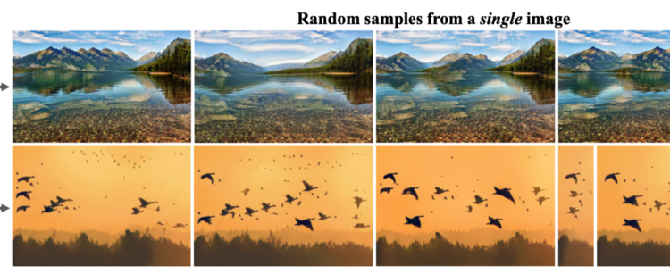
SinGAN is a novel unconditional* generative model that is trained using a single image. Traditionally, GANs have been trained on class-specific datasets and capture common features among images of the same class. SinGAN, on the other hand, learns from the overlapping patches at multiple scales of a particular image and learns its internal statistics. Once trained, SinGAN can produce assorted high-quality images of arbitrary sizes and aspect ratios that semantically resemble the training image but contain new object configurations and structures.

* An unconditional GAN creates samples purely from randomized input, while a conditional GAN generates samples based on a “class label” that controls the type of image generated.

Figure 2. The hierarchical (pyramid) structure of SinGAN.

The SinGAN network contains a hierarchy (pyramid) of generators G and discriminators D:

As shown by the arrows in figure 2, we both train and infer from the coarsest level N to the finest level 0.

When training, we train against the ground truth image pyramid x:

In this image pyramid, level n’s width and height is r times of level n + 1, where r > 1:

We also inject a pyramid of noise z with the same size of x at every level:

Using this hierarchical structure, SinGAN can capture the statistics of complex image structures at different scales, where each pair of G and D is responsible for one scale.

At each scale, we focus on small image patches of a specific size instead of the entire image. We refer to this size as the “effective patch size” shown as yellow rectangles in figure 2. Since the generators and discriminators are both Convolutional Neural Networks, this size is determined by the networks’ receptive fields. In SinGAN, generators and discriminators of different layers share the same structure and thus have the same receptive field (in terms of pixels). And because the generated images get progressively larger in the SinGAN hierarchy, the patch size becomes smaller compared with the generated images.

On coarser levels, we learn and generate big patches that reflect the global properties of the image, which are the arrangement and shape of large objects. For example, sky and ground placements in natural images.
On finer levels, we learn and generate small patches that reflect the local properties of the image, such as details and textures.

Even on coarser levels, the effective patch size is relatively small compared with the training and generated images. This prevents the generator from memorizing the entire image and re-generating it identically.

Generator Structure

Figure 3. Structure of generator G.

All generators share the same structure as shown in figure 3, which can be represented by this formula:

1. Inputs.

The coarsest generator (level N) only accepts a random noise image (usually spacial white Gaussian) as input. In other words, it is purely generative.

Other generators accept a random noise image and the up-sampled generated image from the previous scale.

2. Add noise z to the up-scaled image generated by the previous generator. This step ensures that the GAN does not disregard the noise (a problem in conditional schemes involving randomness).

3. The network ψ is made up of 5 convolutional layers and generates the missing details between layers.

Each layer’s structure is: conv(kernel size: 3, stride: 1, padding: 1) -> batch norm -> leaky ReLU (negative slope: 0.2).

Total receptive field (patch size) of ψ: 11 x 11.

4. A skip connection adds the up-scaled image from the previous generator to the output of the convolutional layers.

Discriminator Structure

We use Markovian discriminators to distinguish between the ground truth and generated patches, as opposed to the entire image. It accepts both the generated image and a down-sampled version of the ground truth image as input. Its architecture is the same as the conv net ψ of generator G.

Injection to Middle Layers

In some of the image manipulation tasks described in the Applications and Results chapter, we do not generate the result completely from noise. Instead, we inject a down-sampled training (ground truth) image into the generation pyramid at scale n, where n < N and feed it through the finer generators:

Figure 4. Injecting a horse image into the middle layers of a trained zebra model.

In figure 4, we train the SinGAN model on the zebra image (bottom right) and feed a down-sampled horse image (bottom left) into the generator Gn (in this case n = 6 while N = 9). As this image propagates through the generation pyramid, stripes are gradually added to the horse, which grants it the appearance of a Zebra.

Figure 5. Comparison of injection levels.

As shown in figure 5, the coarser the injection level, the larger structures SinGAN will modify to match the statistics of patches in the generated image to the training image. If we want to keep the global structure of the generated image, we must inject at a finer scale.

We train one GAN at a time from the coarsest level (N) to the finest level (0). Once a GAN is trained, it is kept fixed to train finer-levelled GANs.

The total loss function is:

where Ladv and Lrec refer to adversarial loss and reconstruction loss respectively.

Background: Wasserstein GAN (WGAN)

Traditionally, GAN loss functions used to quantify the similarity between the generated data distribution (pg) and the real sample distribution (pr) by JS Divergence when the discriminator is optimal.

Yet this approach has some problems. First of all, the dimensions of many real-world datasets (pr) only appear to be artificially high and tend to concentrate in a lower-dimensional manifold due to the object’s intrinsic properties. For example, a cat must have four legs, while a bird must have two legs, etc. It also turns out that the dimensions of generated datasets (pg) usually lie in low dimensional manifolds. Since input (noise z) dimensions are usually much smaller than the generated images’ dimensions, it is unlikely that the results can fill up high-dimensional spaces.

Figure 6. Low-dimensional manifolds in high-dimension space can hardly have overlaps.

When two low-dimensional manifolds lie in a high-dimensional space, they are likely to be disjoint. Figure 6 gives an example of 1D lines and 2D surfaces lying in 3D space where they barely intersect.

Figure 7. An extreme case of two degenerate distributions.

Let’s consider the case in figure 7 where two degenerate distributions are completely disjointed and have distance θ on the x-axis. As long as the distributions are disjointed from each other, JS Divergence always produces a constant value:

This value does not reflect the magnitude of disjoint and is thus not meaningful. Besides, when θ = 0, JS Divergence is not differentiable (not smooth).

Wasserstein GAN, on the other hand, uses Wasserstein Distance to measure the similarity between pg and pr. This distance is also known as “Earth Mover’s Distance” because it represents the minimum energy cost of moving and transforming a pile of dirt in the shape of one probability distribution to the shape of the other distribution. The cost here is defined as the amount of dirt moved multiplied by the distance moved.

* In the formula above, inf means infimum (greatest lower bound). Π(p, q) is the set of all possible joint probability distributions between p and q. Joint distributions γ ∈ Π(p , q) describe dirt transport plans in the continuous probability space.

In the previous example where two distributions are completely disjointed, Wasserstein Distance is meaningful:

In addition to providing a meaningful distance for the example above, the Wasserstein metric also produces a smooth measure, which is super helpful for a stable learning process using gradient descent.

Adversarial Loss

The adversarial loss penalizes for the distance between the distribution of patches in the ground truth image and the generated samples. In this model, we use the WGAN loss introduced above with gradient penalty. The final discrimination score is the average over the patch discrimination map. That is, we define the loss for the whole image rather than over random crops. This allows the network to better learn boundary conditions since those boundary patches and paddings are included in the loss.

Reconstruction Loss

The reconstruction loss makes sure that there exists a set of noise maps that can reproduce the ground truth image. In particular, we set the noises of all layers except for the coarsest layer to zero when calculating this loss:

Using the noise map above, we define the reconstruction loss as the distance between the image generated from the noise z* and the ground truth (training) image:

For the coarsest (level N) layer, we have:

We may use reconstruction loss to determine the amount of details that need to be added at a specific scale. In practice, we determine the standard deviation σn of noise zn by calculating the RMS error between an up-scaled previous layer output and the ground truth image of the current layer:

In addition to that, zrec is also used for “Single Image Animation” purposes.

Generate Similar Images

Figure 8. Generate similar images.

This is SinGAN’s main application. By feeding noises of arbitrary size and aspect ratio into the network, we may generate realistic image samples that preserve the original patch distribution but have new object configurations and structures.

Super Resolution (SR) Image

Figure 9. Super Resolution Image.

Up-scales a Low Resolution (LR) image by a factor s, where s > 1.

Firstly, we train the network on the LR image. No SR images are required for training (a significant difference from traditional solutions).

We choose a pyramid scale factor r = k√s (level n’s width and height is r times of level n + 1), where k is an arbitrary positive integer.
Since we want the SR image to be as faithful as possible, we use a very big reconstruction loss weight α = 100.

After training, we generate the SR image by doing the following steps for k times:

Up-scale the LR image by r.
Inject it to the last (finest) generator G0 for k times.

Paint-to-Image (Style Transfer)

Figure 10. Paint to image.

Transfers a clip-art into a photo-realistic image.

We first train the network on the photo-realistic image itself. Then we down-sample the clip-art and feed it into a coarse scale (like N — 1 or N — 2) of the SinGAN pyramid. Ideally, the global structures of the clip-art are preserved and the fine details are added with high fidelity.

Figure 11. SinGAN’s failure on highly textured photo-realistic images.

Unfortunately, the SinGAN model does not deal well with highly textured photo-realistic images in this application. This is because the network was only exposed to textured images during training and may fail to handle clip-arts that are too smooth compared with the training data. One possible workaround is to train the last generator using quantized* input from the previous generator.

* Quantization: Reduces the number of colors used in the image.

Harmonization (Blending / Pasting Objects)

Figure 12. Harmonization.

Blends a (possibly alien) object naturally with a background image.

As usual, we train the network on the background image. After that, we naively paste the alien object to the background image and inject a down-sampled version of this composite to the network. As mentioned in the “Injection to Middle Layers” chapter, the coarser the injection level, the larger structures SinGAN will modify to match the statistics of patches in the generated image to the training image.

Editing (Copy and Paste Patch)

Figure 13. Editing.

Copies part of an image to another position realistically. The process is identical to Harmonization, except that the naively pasted object is from the image itself.

Single Image Animation

Demo: https://youtu.be/xk8bWLZk4DU

Creates a short video clip with realistic object motion from a single input image.

We train the network with a large reconstruction loss weight α = 100. Then we start with the reconstruction noise zrec and generate the animation using a random walk in noise (z) space.

Tamar Rott Shaham, Tali Dekel, Tomer Michaeli. SinGAN: Learning a Generative Model from a Single Natural Image. arXiv:1905.01164, 2019.
Ishaan Gulrajani, Faruk Ahmed, Martin Arjovsky, Vincent Dumoulin, Aaron C Courville. Improved training of Wasserstein GANs. In Advances in Neural Information Processing Systems, pages 5767–5777, 2017.
Ishaan Gulrajani, Faruk Ahmed, Martin Arjovsky, Vincent Dumoulin, Aaron Courville. Improved Training of Wasserstein GANs. arXiv:1704.00028, 2017.
Lilian Weng. From GAN to WGAN. arXiv:1904.08994, 2019.
Wengling Chen, James Hays. Sketchygan: towards diverse and realistic sketch to image synthesis. In Proceedings of the IEEE Conference on Computer Vision and Pattern Recognition, pages 9416–9425, 2018.
Generative adversarial network. In Wikipedia. Retrieved from https://en.wikipedia.org/wiki/Generative_adversarial_network