2.1 Understanding the train data:
1. Id — Unique identifier of row.
2. Query — Text about the query.
3. Product_title — Text about the title of the product.
4. Product_description — Text about the product description.
5. Median_relevance — Median relevance score given by 3 raters
6. relevance_variance — Variance of the relevant scores given by these three raters.
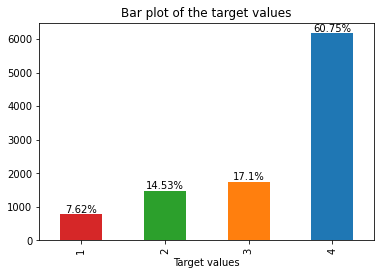
Let us visualize the target values distribution:

Observation:
- Data is very imbalanced. Most of the data points are from class — 4. Very few data points belong to class — 1
2.2 Check for NAN values.
ax = missingno.matrix(df)
print('Percentage of points that are having missing values',round(sum(df.product_description.isna())/df.shape[0]*100,2),'%')
Percentage of points that are having missing values 24.06 %
# I cannot just drop the 24.06% of the points randomly.
# I will fill the missing values with an empty string
df.product_description.fillna('',inplace=True)
2.3 Data Analysis of the feature ‘Query’
Let us check do we have any repetition of text in the query column:
df['query'].value_counts()
Visualize the lengths of the query sentence:

Analysis of Query text:
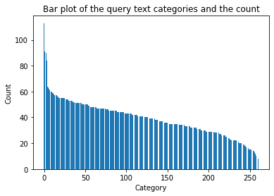
- Total 261 unique categories → We can do any categorical encoding on this column.
- Most of the categories are repeated in the range 30–50 times
- Wireless mouse is the most common query occurring 113 times in the data and Dollhouse bathtub was present the least times in the data — 8 times
2.4 Data Analysis of the feature ‘Product_title’
Let us see some stats about the feature product_title
Visualizing the length of the sentences:
product_title_len = df.product_title.str.len()
plt.plot(sorted(product_title_len))
Going one more step deeper,
Do the length of the sentence and the target variable have any relation?
sns.histplot(data = df, x = 'product_title_len', y = 'median_relevance')
Analysis:
- The more the count of common words between query and product title the higher the chance of getting a strong rating.
- We cannot draw any analysis based on only the product title length as all the classes are overlapping.
- Simple text data → We can do TFIDF, W2V and TFIDF_W2V on this column.
2.5 EDA Product Description:
Let us visualize the lengths of the sentences
Going one more step deeper,
start = 99.9
for i in range(10):
print('{:.2f}th percentile value is {:.1f}'.format(start,np.percentile(df.product_description_len,start)))
start+=0.01
out= sum(df.product_description_len>10**3)
print('{} product titles have length>145 i.e greater than 99.96 percentile'.format(out))
When we see the count of common words from product_description and product_title even though there are more than 40 common words the median_relevancy is almost equally distributed.
Note: The number of datapoints for class- 4 are very high and hence just looking at the above graph and coming to a decision that higher the common words in product_title and product_description the better the relevancy is not right as the count between the classes is not differing by much.
2.6 Checking for HTML values:
check_html(df[‘query’])
# Output
Time take to run is 0:00:00.861348
Number of rows with html code 0check_html(df[‘product_title’])
# Output
Time take to run is 0:00:01.067391
Number of rows with html code 0check_html(df[‘product_description’])
# Output
Time take to run is 0:00:00.730124
Number of rows with html code 94
It is important to check for the presence of HTML tags in text data and more importantly which column has HTML tags. So, we can only work on removing HTML tags only from that particular column. If you are working on a large dataset, this will definitely save some time.
2.7 Understanding the test data:
The test data given by Kaggle is large it has 22513 datapoints and it might have a lot of artificial values just to be ignored during evaluation. There is no relevance_variance column in test data.
3. Performance metric:
Here the target variables are ordinal in nature. We cannot use simple classification metrics like accuracy or F1-score. As shown below:
So, accuracy needs exact class labels for higher scores so, even though the class labels are close to actual data it will give us the same results.
But kappa score will give better results if the predicted classes are close to the actual train data. For more details of how to implement the quadratic kappa score, I recommend checking this nice Kaggle kernel.
You might be thinking why not MSE. FYI, MSE in case-1 will return 7.5 and in case-2 will return 1. For improving Kappa score you can do two things:
- Build a regression model that reduces MSE, it was observed that reduced MSE gives a better Kappa score. After training, we can round off to the nearest integer to get the class label.
Choosing thresholds:
As the regression can take any value from 0 to infinity, you can say everything below 0.5 is class 0, between 0.5 and 1.5 is class 1, between 1.5 and 2.5 is class 2, between 2.3 and 3.5 is class 3 and everything above 3.5 is class 4.
Thus the coefficients are : [0.5, 1.5, 2.5, 3.5]
These coefficients may or may not be optimal. Remember, we are trying to have the best coefficients that bring an improvement to evaluation metric. You can get the best coefficients using this kernel.
2. Use Kappa score directly as the loss function. (This might be hard to do)
4. First cut approach:
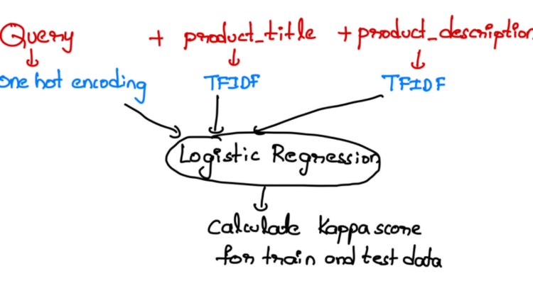
Now we know more about the data the simplest approach is to convert the Query into the vector using one-hot encoding and text data(product_title and product_description) into numerical form and fit a baseline model like Logistic regression.
You can also try Linear regression and round off the results to the nearest integer.
5. Text Preprocessing:
5.1 Clean the HTML
Beautiful soup has made life easy and with just two lines of code you can remove HTML tags from a string.
5.2 Word replacement:
Words with similar meaning are replaced with a common word, for example:
This list is taken from the winner solution of this competition, thanks to the author we took his time in finding these nuanced differences in data.
5.3 Stemming, decontraction and stop word removal:
These are the common techniques you will do in any NLP problem, you can find the code below:
5.4 Summarize the processing steps:
HTML tag removal →word replacement →stemming →decontraction →removing punctuation marks →stop words removal
Is preprocessing necessary, what will it bring to us?
Here is a glimpse of the percentage of data points where there is 100% match between query and title before and after preprocessing.
As you can notice without preprocessing there is 41% of data points where all the words in query are present in the title, but after preprocessing it is increased to 49% (in the datapoints having median relevancy as 4).
6. Text vectorization:
Before starting this step make sure you have split the training data properly.
6.1 Handling Query data:
Make sure you replace all the spaces with ‘_’ to create a single category.
# Replacing space with underscore to make it a single word.
df['cleaned_query'] = df.apply(lambda x : x['query'].replace(' ','_'),axis = 1)
Code to do one-hot encoding on cleaned_query column.
If you do not replace space with an underscore then the count vectorizer
- Will treat each word as a unique feature, say in the datapoint ‘wireless mouse’, we do not want ‘wireless’ to be a feature and ‘mouse’ to be separate a feature, we want the combination should be unique.
2. Increases the dimension of the data unnecessarily.
6.2 Handling product_title and product_description using TFIDF vectorizer
For both of these data points we will do simple TFIDF vectorization, here is the code for product_title you can follow the same approach for product_description.
6.3 Handling product_title and product_description using average W2V:
In this section we will be creating a word to vector model for our text data, the pre-trained word embedding can be downloaded from this link.
In the below code first, we are loading the glove vectors and now for each word in each sentence if the word embedding is present in the glove file then get the vector(model.get(<word>)). Based on the number of embedding present we calculate the average.
Note: Make sure you are not doing stemming while using word to vectors as stemming can result in a different form of a word and this word can be non-English. For example, the stem(‘batteries’) will give me ‘batteri’ and this word will not be present in the word-embedding file.
Any other solution?
Yes, you can do Lemmatization to solve the problem as it returns an actual English word.
6.4 Handling text data using TFIDF-W2V:
Instead of taking a simple average of the word-embeddings, we will multiply with the corresponding TFIDF value and then take the average of the word-embeddings.
7. Advanced feature engineering.
Let C — All the combinations of the query, title and description — (query, title),(title, description),(description, query).
- Total word counts in each of the text feature.
- Common word counts in C.
- Unique common word counts in C.
- Normalized Common word counts — Divide the common words with the number of words between the maximum of words between two columns.
- Common bigrams count in C, unique bigrams count and all possible ratios in the features of C.
- Common trigrams count in C, unique bigrams count and all possible ratios in the features of C.
- Count the digits in Query, Description, Query.
8. Modelling:
8.1 Base line model:
Let us try with the first cut approach:
There are many combinations to try, to save some time I am using the kernel directly on the data I have generated.
I got 0.612 as the Kappa score for the test data but this score can be significantly improved with stacking more complex models.
References:
