Explore One-Class SVM for Anomaly detection
This post is the second in the series; here you will explore One-Class SVM, a semi-supervised technique for anomaly detection.
Anomaly Detection Techniques: Part 1- Understand Inter-Quartile Range, Elliptic Envelope, and Isolated Forest
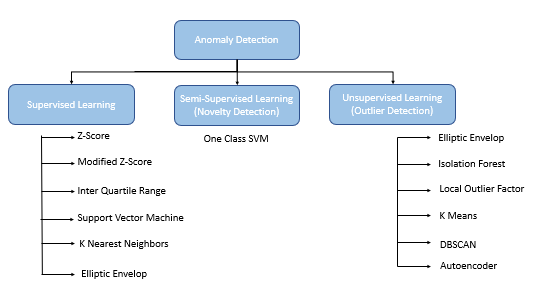
Anomaly detection using Machine Learning can be divided into Supervised, Semi-Supervised, or Unsupervised algorithms.
- Supervised Anomaly Detection: A labeled dataset with inliers and outlier data points where learning happens based on the labeled dataset used for training.
- Semi-Supervised Anamoly Detection(Novelty Detection): Outliers do not pollute training data, and the anomaly detection algorithm only detects if the new observation is an inlier or an outlier. Built on the premise that outliers can form a high-density cluster as long as the normal data points in the training dataset form a low-density cluster
- Unsupervised Anomaly Detection(Outlier Detection): An unlabeled dataset containing both inlier and outlier data points. These algorithms are built on the premise that inlier data points form high-density clusters and anomalies or outliers are located in low-density regions.
One Class Support Vector Machine(OCSVM)
One Class SVM is a novelty anomaly detection algorithm based on the premise that the training data is not polluted by the outliers and a new observation is detected as an inlier or an outlier. OCSVM is applied for binary classification
OCSVM assumes that anomalies can form dense clusters as long as they form a low-density region in the training dataset.
OCSVM mode is trained in only one class, referred to as the normal class. The model learns all the features and patterns of the normal class . When a new observation is introduced to the model, then based on its learning, the OCSVM detects if the new observation deviates from the normal behaviour then it classifies it as an oulier else the new observation will identified as an inlier.
OCSVM is based on Support Vector Machines where the binary classes are separated by a non-linear hyper plane
Dataset used in this post is Breast Cancer Winsoncin data from UCI.
Here we apply the One-Class SVM in an unsupervised mode.
Importing required libraries
from sklearn.svm import OneClassSVM
import pandas as pd
from sklearn.decomposition import PCA
from mpl_toolkits.mplot3d import Axes3D
from sklearn.preprocessing import StandardScaler
import numpy as np
from matplotlib import pyplot as plt
from numpy import quantile, where, random
from sklearn.metrics import confusion_matrix, accuracy_score, precision_score, recall_score
from sklearn.model_selection import train_test_split
%matplotlib inline
Read the dataset
#Set the path of the dataset and read the dataset
DATASET_PATH=r'breast-cancer-wisconsin.data.csv'
dataset= pd.read_csv(DATASET_PATH)
# Cleaning teh data and replacing ? with a 0
dataset['Bare Nuclei'] = dataset['Bare Nuclei'].replace('?', 0)
dataset.loc[dataset['Class'] ==4, 'normal'] = -1
dataset.loc[dataset['Class'] ==2, 'normal'] = 1
dataset.head(2)
Creating training and test dataset
We use 80% of the data for training and the rest of the 20% data for test, also creating the input and the target variables for training.
train_rec_count=int(len(dataset)*.8)
dataset_train= dataset.iloc[:train_rec_count,:]
normal_rec_count=len(dataset_train.loc[dataset_train['Class']==2])
dataset_test=dataset.iloc[train_rec_count:,:]
dataset_test = dataset_test.reset_index()
dataset_test.drop(columns='index', axis=1, inplace=True)
X_train= dataset_train.iloc[:, 1:10]
y_train= dataset_train.iloc[:, 11]
X_test=dataset_test.iloc[:, 1:10]
Create the One-Class Support Vector Machine
#Creating the One-Class Support Vector Macinenu_percentage= (train_rec_count-normal_rec_count)/train_rec_count
ocsvm = OneClassSVM( nu=nu_percentage)
nu: by default, the value is 0.5. It represents the fraction of training errors and can be between 0 and 1. Here we specify the anomaly percentage in the training dataset.
Fitting the training data and predicting the results for the test data
ocsvm.fit(X_train, y_train)
yhat=ocsvm.predict(X_test)
To run the OCSVM in unsupverised mode, just provide the input features
ocsvm.fit(X_train)
Evaluating the performance of the model
dataset_test['onesvm_anomaly']=yhat
cm=confusion_matrix(dataset_test['normal'], dataset_test['onesvm_anomaly'])print(" Accuracy Score for One-Class SVM :", accuracy_score(dataset_test['normal'], dataset_test['onesvm_anomaly']))
print(" Precision for One-Class SVM :", precision_score(dataset_test['normal'], dataset_test['onesvm_anomaly']))
print(" Recall for One-Class SVM :", recall_score(dataset_test['normal'], dataset_test['onesvm_anomaly']))
print(" Confusion Matrix: n", cm)
Plotting a 3-D plot for inliers and outliers
Reduce the dimensionality of the input features for test data using PCA
pca= PCA(n_components=3)
scaler= StandardScaler()
X_scaled=scaler.fit_transform(X_test)
X_reduced=pca.fit_transform(X_test)
Plotting the inliers and outliers on the original test dataset, p, and the predictions made by One-Class SVM
original_anomaly_index=dataset_test.loc[dataset_test['normal']==-1]
original_anomaly_index=list(original_anomaly_index.index)
ocsvm_anomaly_index=dataset_test.loc[dataset_test['onesvm_anomaly']==-1]
ocsvm_anomaly_index=list(ocsvm_anomaly_index.index)#PLotting the outliers and inliersfig=plt.figure(figsize=(15, 5))
ax= fig.add_subplot(121, projection='3d')
ax.scatter(X_reduced[:,0],X_reduced[:,1], zs=X_reduced[:,2], s=4, lw=1, label='inlier', c="green", marker="o")
ax.scatter(X_reduced[original_anomaly_index,0],X_reduced[original_anomaly_index,1], zs=X_reduced[original_anomaly_index,2], lw=2, s=60, marker="x", c="red", label="outliers")
ax.legend(loc='lower left')
plt.title('Outliers on Original scaled data')
ax= fig.add_subplot(122, projection='3d')
ax.scatter(X_reduced[:,0],X_scaled[:,1], zs=X_reduced[:,2], s=4, lw=1, label='inlier', c="green")
ax.scatter(X_reduced[ocsvm_anomaly_index,0],X_reduced[ocsvm_anomaly_index,1],X_reduced[ocsvm_anomaly_index,2], lw=2, s=60, marker="x", c="red", label="outliers")
ax.legend(loc='lower left')
plt.title('Outliers based on One-class SVM')
plt.show()
Conclusion:
One-Class Support Vector Machine is a novelty anomaly detection algorithm that is based on Support Vector Machine. It can be used as both a supervised and unsupervised algorithm. the outliers do not pollute the training data
References:
https://scikit-learn.org/stable/modules/outlier_detection.html