Basics: Gradient*Input as Explanation

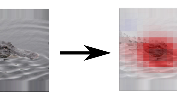
In this post, I want to get to the basics of gradient-based explanations, how you can use them, and what they can or can’t do.

Gradient*Input is a great way to explain differentiable machine learning models, such as neural networks, because it is conceptually simple and easy to implement. Computing gradients is also very fast, especially if you make use of modern ML libraries, like pytorch, TensorFlow, or JAX, that include automatic differentiation.

Gradient*Input is only suitable for explaining relatively simple models, but it is an essential concept, necessary to understand a host of other gradient-based techniques that are more robust.

Chances are you have come across gradients in high-school or university classes. This will not be a rigorous introduction, but just a quick reminder.

First, we need to remember what derivatives are. In essence, the derivative of a differentiable function, f(x): ℝ → ℝ, tells us for any input x how much f(x) will change if we increase x a little bit.

This is useful for example for convex optimization problems: To find a minimum we just start at any point and go into the direction in which f(x) decreases the most and repeat calculating the gradient and taking steps until we arrived at the minimum, i.e. gradient descent.

The gradient of a differentiable function f(x): ℝ^d → ℝ is just a vector of (partial) derivatives of f(x) w.r.t. to every of the d dimensions of x.

The gradient tells us for any point (x1,x2) how much f(x1, x2) will change when taking a small step in any direction in the d-dimensional input space. Thus, it also tells us in what direction f(x1, x1) will increase the most.

Formally, we write the gradient of f(x) w.r.t. x as ∇f(x).

A large class of explanation methods meant to explain machine learning models is called attribution methods, producing explanations called attributions. The purpose of an attribution is to attribute a share of the responsibility for a particular output to every dimension of the respective input.

For example, consider a DNN trained to recognize crocodiles from an image. An attribution method would assign a score to every pixel of the input, indicating how much this pixel contributed to the final output (crocodile or not-crocodile). If we put these individual attributions back together into a matrix, we typically call them an attribution map. We can visualize an attribution map as an image, indicating which regions of the image are important.

There are different ways of creating attribution maps and generally, there is no ground-truth to tell us which pixel contributed how much to the output. That is why no attribution method can claim it is “the right one”. Generally, they all have different properties that may be useful in different application scenarios.

Gradient*Input is one attribution method, and among the most simple ones that make sense. The idea is to use the information of the gradient of a function (e.g. our model), which tells us for each input dimension whether the function will increase if we take a tiny step in this direction. If our function output is, say, the probability of the image containing a crocodile, then the gradient basically tells us how much each dimension increases the model’s prediction of crocodileness.

Now, if we know for each dimension how much one step in this direction increases the output, we just need to multiply it with the input itself to get a complete attribution.

The idea is that the gradient tells us the importance of a dimension, and the input tells us how strongly this dimension is expressed in the image. Putting this together, the attribution for a dimension is only high if 1) the dimension seems to be important for the output and 2) the value for the dimension is high.

So far, it seems all very reasonable. There is only one problem: the gradient only tells us the importance of a dimension if we just take a tiny step. This is very local information, and when explaining complex functions, the gradient can change quickly even after a few tiny steps in the input space. This means that the function might go up if we take a step in the gradient direction, but it might also go down if we take a larger step in the same direction — effectively invalidating the explanation provided by gradients.

Now that sounds pretty disappointing and there are certainly datasets and models for which Gradient*Input does better than for others. If you are trying to explain a shallow neural network, it is still worth a try.

There are remedies to this problem though, which rely on the same principle as Gradient*Input but make it more robust. Perhaps the simplest are SmoothGrad and Integrated Gradients but there are countless other methods out there that are more sophisticated and may build on different principles.

Gradient*Input’s strength that it is so simple and fast. It is also a solid conceptual basis for more involved explanation methods.

The downside of vanilla gradients as an explanation method is that they are only suitable to explain a function locally. This means, that you should only use them to explain rather simple functions because simplicity implies that they behave similarly globally as they do locally.

In one of my previous posts, I made a comparison of gradient-based explanation methods. All of them are based on Gradient*Input, and adapt it to be more suitable for explaining complex functions.

Of course, there are many more explanation methods out there. The most popular ones include Occlusion Analysis, SmoothGrad, Integrated Gradients, Expected Gradients, LRP, DeepLIFT, and Shapley Values. I would suggest turning to them if you want to explain deep neural networks.

I hope you learned something useful.