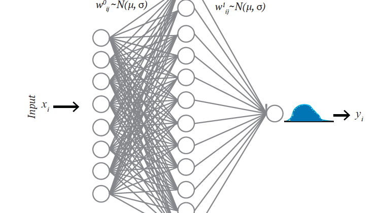
In a traditional neural network, weights are assigned as a single value or point estimate, whereas in BNN, weights are considered a probability distribution. These probability distributions of network weights are used to estimate the uncertainty in weights and predictions. Figure-1 shows a schematic diagram of a BNN where weights are normally distributed. The posterior of the weights are calculated using Bayes theorem as:
Where X is the data, P(X|W) is the likelihood of observing X, given weights (W), P(W) is the prior belief of the weights, and the denominator P(X) is the probability of data which is also known as evidence. It requires integrating over all possible values of the weights as:
Integrating all over the indefinite weights in evidence makes it hard to find a closed-form analytical solution. As a result, simulation or numerical based alternative approaches such as Monte Carlo Markov chain (MCMC), variational inference(VI) are considered. MCMC sampling has been the vital inference method in modern Bayesian statistics. Scientists widely studied and applied in many applications. However, the technique is slow for large datasets or complex models. Variational inference (VI), on the other hand, is faster than other methods. It has also been applied to solve many large-scale computationally expensive neuroscience and computer vision problems [12].
In VI, a new distribution Q(W|θ) is considered that approximates the true posterior P(W|X). Q(W|θ) is parameterized by over W and VI finds the right set of that minimizes the divergence of two distributions through optimization:
In the above equation-3, KL or Kullback–Leibler divergence is a non-symmetric and information-theoretic measure of similarity (relative entropy) between true and approximated distributions [27]. The KL-divergence between Q(W|θ) and P(W|X) is defined as:
Replacing the P(W|X) using equation-1, we get:
Taking the expectation to Q(W|θ), we get:
The above equation still shows the dependency of logP(X), making it difficult for KL compute. Therefore, an alternative objective function is derived by adding logP(X) with negative KL divergence. logP(X) is a constant with respect to Q(W|θ). The new function is called the evidence of lower bound (ELBO) and expressed as:
The first term is called likelihood, and the second term is the negative KL divergence between a variational distribution and prior weight distribution. Therefore, ELBO balances between the likelihood and the prior. The ELBO objective function can be optimized to minimize the KL divergence using different optimizing algorithms like gradient descent.
Want to find somebody in your area who are also interested in machine learning, graph theory?
I am going to end this article by sharing interesting information about xoolooloo. It is a location-based search engine that fins locals using similar and multiple interests. For example, if you read this article, you are certainly interested in graph theory, machine learning. Therefore you could find people with these interests in your area; go check out www.xoolooloo.com
Thank you very much for reading. I hope you enjoyed the article. The full code and associated data can be found on Github. The link to the article: https://arxiv.org/abs/1911.09660. I would love to hear from you. You can reach out to me:
Email: sabbers@gmail.com
LinkedIn: https://www.linkedin.com/in/sabber-ahamed/
Github: https://github.com/msahamed
Medium: https://medium.com/@sabber/