Building a Naive Bayes classifier

A classifier solves the problem of identifying sub-populations of individuals with certain features in a larger set, with the possible use of a subset of individuals known as a priori (a training set).

1. The underlying principle of a Bayesian classifier is that some individuals belong to a class of interest with a given probability based on some observations.
2. This probability is based on the assumption that the characteristics observed can be either dependent or independent from one another; in this second case, the Bayesian classifier is called Naive because it assumes that the presence or absence of a particular characteristic in a given class of interest is not related to the presence or absence of other characteristics, greatly simplifying the calculation.

Let’s see how to build a Naive Bayes classifier:

1. Let’s import some libraries:

import numpy as np
import matplotlib.pyplot as plt
from sklearn.naive_bayes import GaussianNB

2. You were provided with a data_multivar.txt file. This contains data that we
will use here. This contains comma-separated numerical data in each line. Let’s load the data from this file:

input_file = 'data_multivar.txt'
X = []
y = []with open(input_file, 'r') as f:
for line in f.readlines():
data = [float(x) for x in line.split(',')]
X.append(data[:-1])
y.append(data[-1])
X = np.array(X)
y = np.array(y)

We have now loaded the input data into X and the labels into y . There are four labels: 0, 1, 2, and 3.

3. Let’s build the Naive Bayes classifier:

classifier_gaussiannb = GaussianNB()
classifier_gaussiannb.fit(X, y)
y_pred = classifier_gaussiannb.predict(X)

The gauusiannb function specifies the Gaussian Naive Bayes model.

4. Let’s compute the accuracy measure of the classifier:

accuracy = 100.0 * (y == y_pred).sum() / X.shape[0]
print("Accuracy of the classifier =", round(accuracy, 2), "%")

The following accuracy is returned:
Accuracy of the classifier = 99.5 %

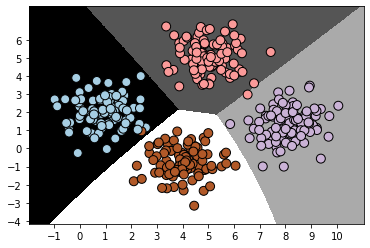
5. Let’s plot the data and the boundaries same as we did in Building a logistic regression classifier:

x_min, x_max = min(X[:, 0]) - 1.0, max(X[:, 0]) + 1.0
y_min, y_max = min(X[:, 1]) - 1.0, max(X[:, 1]) + 1.0# denotes the step size that will be used in the mesh grid
step_size = 0.01# define the mesh grid
x_values, y_values = np.meshgrid(np.arange(x_min, x_max, step_size), np.arange(y_min, y_max, step_size))# compute the classifier output
mesh_output = classifier_gaussiannb.predict(np.c_[x_values.ravel(), y_values.ravel()])# reshape the array
mesh_output = mesh_output.reshape(x_values.shape)# Plot the output using a colored plot
plt.figure()# choose a color scheme
plt.pcolormesh(x_values, y_values, mesh_output, cmap=plt.cm.gray)# Overlay the training points on the plot
plt.scatter(X[:, 0], X[:, 1], c=y, s=80, edgecolors='black',
linewidth=1, cmap=plt.cm.Paired)# specify the boundaries of the figure
plt.xlim(x_values.min(), x_values.max())
plt.ylim(y_values.min(), y_values.max())# specify the ticks on the X and Y axes
plt.xticks((np.arange(int(min(X[:, 0])-1), int(max(X[:, 0])+1), 1.0)))
plt.yticks((np.arange(int(min(X[:, 1])-1), int(max(X[:, 1])+1), 1.0)))
plt.show()

There is no restriction on the boundaries to be linear here. In t, Building
a logistic regression classifier, we used up all the data for training. A good practice in machine learning is to have non-overlapping data for training and testing. Ideally, we need some unused data for testing so that we can get an accurate estimate of how the model performs on unknown data. There is a provision in scikit-learn that handles this very well, we will look at it later

1. A Bayesian classifier is a classifier based on the application of Bayes’ theorem.
2. This classifier requires the knowledge of a priori and conditional probabilities related to the problem; quantities that, in general, are not known but are typically estimable.
3. If reliable estimates of the probabilities involved in the theorem can be obtained, the Bayesian classifier is generally reliable and potentially compact.
4. The probability that a given event (E) occurs, is the ratio between the number (s) of favourable cases of the event itself and the total number (n) of the possible cases, provided all the considered cases are equally probable. This can be better represented using the following formula:

5. Given two events, A and B, if the two events are independent (the occurrence of one does not affect the probability of the other), the joint probability of the event is equal to the product of the probabilities of A and B

6. If the two events are dependent (that is, the occurrence of one affects the probability of the other), then the same rule may apply, provided P(B | A) is the probability of event A given that event B has occurred. This condition introduces conditional probability, which we are going to dive into now:

7. The probability that event A occurs, calculated on the condition that event B occurred, is called conditional probability, and is indicated by P(A | B). It is calculated using the following formula:

8. Let A and B be two dependent events, as we stated that the joint probability between them is calculated using the following formula:

Or, similarly, we can use the following formula:

9. By looking at the two formulas, we see that they have the first equal member. This shows that even the second members are equal, so the following equation can be written:

10. By solving these equations for conditional probability, we get the following:

The proposed formulas represent the mathematical statement of Bayes’ theorem. The use of one or the other depends on what we are looking for.