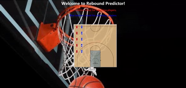
Note:
- The location represents where a player is standing when the shot is thrown, and it is represented by x-y coordinates.
- The X coordinate is measured in feet and represents the distance from the center of the court, length-wise. -47 represents the baseline of the offensive team’s end. 47 represents the baseline of the defending team’s end.
- The Y coordinate is measured in feet and represents the distance from the basket, width-wise. -25 represents the right side of the court, 25 represents the left side of the court (for someone facing the offensive basket).
- In the output, there are empty values which mean that the corresponding shots or free throws are made. Since we only care about the scenarios where there are rebounds, we need to handle this later.
Data Cleaning
To begin with, let’s take out the undesirable row values:
# remove the rows where the shots or free throws were made
train = train[train['f.oreb'].isna()==False]
Next, match the rebounded player id with his position in his team and the team condition (offending/defending):
# target columns is a list containing the input columns' names
target_columns = []
for event in ['off', 'def']:
for i in range(1, 6):
target_columns.append('playerid_' + event + '_player_' + str(i))reb_player_id_df = train[target_columns].eq(train['reb_player_id'], axis = 0)
reb_player_position_df = reb_player_id_df.idxmax(1).where(reb_player_id_df.any(1)).dropna()# encode all players on court
# 1~5 means a player is an offending one while 6~10 means a defending one
position_code = {
'playerid_off_player_1': 1,
'playerid_off_player_2': 2,
'playerid_off_player_3': 3,
'playerid_off_player_4': 4,
'playerid_off_player_5': 5,
'playerid_def_player_1': 6,
'playerid_def_player_2': 7,
'playerid_def_player_3': 8,
'playerid_def_player_4': 9,
'playerid_def_player_5': 10
}
output = reb_player_position_df.apply(lambda x: position_code[x])# reset the index
output = output.reset_index(drop=True)
Now, to many degrees, normalized data usually performs better in machine learning because it reduces the influences from outliers and avoids falling into local optimal points. Thus, since we have a certain range for both x and y coordinates, we could try Min-Max normalizer:
train[[col for col in location_columns if '_y_' in col]] = (25 - train[[col for col in location_columns if '_y_' in col]]) / (25 - (-25))
train[[col for col in location_columns if '_x_' in col]] = (47 - train[[col for col in location_columns if '_x_' in col]]) / (47 - (-47))
Now the data is ready to go!
Model selection
I tried a suite of models that are expected to perform well in probability prediction, including Logistic Regression, Linear Discriminant Analysis, Quadratic Discriminant Analysis, Gaussian Naive Bayesian Classifier, and Multinomial Naive Bayesian Classifier.
# define models
models = [LogisticRegression(n_jobs=-1), LinearDiscriminantAnalysis(), QuadraticDiscriminantAnalysis(), GaussianNB(), MultinomialNB()]
Cross-validation:
names, values = [], []# evaluate each model one by one
# and store their names and log loss values
for model in models:
# get a name for the model
name = type(model).__name__[:15]
scores = evaluate_model(train, LabelEncoder().fit_transform(output), model)
# output the results
print('>%s %.3f (+/- %.3f)' % (name, np.mean(scores), np.std(scores)))
names.append(name)
values.append(scores)
The result shows that Linear Discriminant Analysis outperforms all other counterparts, so I selected it as my kernel algorithm.
# save the model
dump(LDA, 'LDA.joblib')
