The number of clusters as one of the input parameters
When we discussed the k-means algorithm, we saw that we had to give the number of clusters as one of the input parameters. In the real world, we won’t have this information available. We can definitely sweep the parameter space to find out the optimal number of clusters using the silhouette coefficient score, but this will be an expensive process! A method that returns the number of clusters in our data will be an excellent solution to the problem. DBSCAN does just that for us.
We will perform a DBSCAN analysis using the sklearn.cluster.DBSCAN
function. We will use the same data that we used in the previous Evaluating the performance of clustering algorithms ( data_perf.txt ) which can be downloaded from here https://github.com/appyavi/Dataset
Let’s see how to automatically estimate the number of clusters using the DBSCAN algorithm:
- import the necessary packages:
from itertools import cycle
import numpy as np
from sklearn.cluster import DBSCAN
from sklearn import metrics
import matplotlib.pyplot as plt
2. Load the input data from the data_perf.txt file.
# Load data
input_file = ('data_perf.txt')
x = []
with open(input_file, 'r') as f:
for line in f.readlines():
data = [float(i) for i in line.split(',')]
x.append(data)
X = np.array(x)
3. We need to find the best parameter, so let’s initialize a few variables:
# Find the best epsilon
eps_grid = np.linspace(0.3, 1.2, num=10)
silhouette_scores = []
eps_best = eps_grid[0]
silhouette_score_max = -1
model_best = None
labels_best = None
4. Let’s sweep the parameter space:
for eps in eps_grid:
# Train DBSCAN clustering model
model = DBSCAN(eps=eps, min_samples=5).fit(X)
# Extract labels
labels = model.labels_
5. For each iteration, we need to extract the performance metric:
# Extract performance metric
silhouette_score = round(metrics.silhouette_score(X, labels),4)
silhouette_scores.append(silhouette_score)
print("Epsilon:", eps, " --> silhouette score:",silhouette_score)
6. We need to store the best score and its associated epsilon value:
if silhouette_score > silhouette_score_max:
silhouette_score_max = silhouette_score
eps_best = eps
model_best = model
labels_best = labels
output:
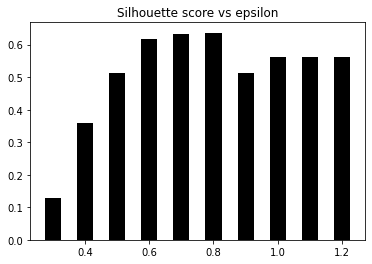
Epsilon: 0.3  --> silhouette score: 0.1287
Epsilon: 0.39999999999999997  --> silhouette score: 0.3594
Epsilon: 0.5  --> silhouette score: 0.5134
Epsilon: 0.6  --> silhouette score: 0.6165
Epsilon: 0.7  --> silhouette score: 0.6322
Epsilon: 0.7999999999999999  --> silhouette score: 0.6366
Epsilon: 0.8999999999999999  --> silhouette score: 0.5142
Epsilon: 1.0  --> silhouette score: 0.5629
Epsilon: 1.0999999999999999  --> silhouette score: 0.5629
Epsilon: 1.2  --> silhouette score: 0.5629
7. Let’s now plot the bar graph, as follows:
# Plot silhouette scores vs epsilon
plt.figure()
plt.bar(eps_grid, silhouette_scores, width=0.05, color='k', align='center')
plt.title('Silhouette score vs epsilon')
plt.show()# Best params
print("Best epsilon =", eps_best)
Output: Best epsilon = 0.7999999999999999
8. Let’s store the best models and labels:
# Associated model and labels for best epsilon
model = model_best
labels = labels_best
9. Some datapoints may remain unassigned. We need to identify them, as follows:
# Check for unassigned datapoints in the labels
offset = 0
if -1 in labels:
offset = 1
10. Extract the number of clusters, as follows:
# Number of clusters in the data
num_clusters = len(set(labels)) - offset
print("Estimated number of clusters =", num_clusters)
output: Estimated number of clusters = 5
11. We need to extract all the core samples, as follows:
# Extracts the core samples from the trained model
mask_core = np.zeros(labels.shape, dtype=np.bool)
mask_core[model.core_sample_indices_] = True
12.Let’s visualize the resultant clusters. We will start by extracting the set of unique labels and specifying different markers:
# Plot resultant clusters
plt.figure()
labels_uniq = set(labels)
markers = cycle('vo^s<>')
13. Now let’s iterate through the clusters and plot the datapoints using different markers:
for cur_label, marker in zip(labels_uniq, markers):
# Use black dots for unassigned datapoints
if cur_label == -1:
marker = '.'
# Create mask for the current label
cur_mask = (labels == cur_label)cur_data = X[cur_mask & mask_core]
plt.scatter(cur_data[:, 0], cur_data[:, 1], marker=marker, edgecolors='black', s=96, facecolors='none')
cur_data = X[cur_mask & ~mask_core]
plt.scatter(cur_data[:, 0], cur_data[:, 1], marker=marker, edgecolors='black', s=32)
plt.title('Data separated into clusters')
plt.show()
- DBSCAN works by treating datapoints as groups of dense clusters.
- If a point belongs to a cluster, then there should be a lot of other points that belong to the same cluster.
- One of the parameters that we can control is the maximum distance of this point from other points. This is called epsilon.
- No two points in a given cluster should be further away than epsilon.
- One of the main advantages of this method is that it can deal with outliers. If there are some points located alone in a low-density area, DBSCAN will detect these points as outliers as opposed to forcing them into a cluster.
DBSCAN presents the following pros and cons:
PROS:
- It does not require to know the number of a priori clusters.
- It can find clusters of arbitrary forms.
- It requires only two parameters.
CONS:
- The quality of clustering depends on its distance measurement.
- t is not able to classify datasets with large differences in density.
