Here i give you details about how google manages such a large set of queries with so much efficiency. And the credit goes to one and only google Page rank algorithm
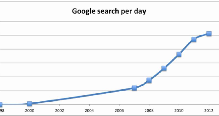
In the year 1998 google handled 9800 average searches per day, in 2012 it shot up to 5.13 billion searches per day. The graph below shows the astronomical growth.
The major reason for google’s success is its page rank algorithm
- Page rank determines how trustworthy and reputable a given website is. But there is also another part.
The input query entered by the user should be used to match the relevant documents and score them. Here we focus on the second part.
Let’s consider three documents to show how this works. Take some time to go through them.
- Document 1 : The game of life is a game of everlasting learning
- Document 2 : The unexamined life is not worth living
- Document 3 : Never stop learning
Let us imagine that you are doing a search on these documents with following query: “ life learning”
The query is a free text query. It means a query in which the terms of query are typed freeform into the search interface , without any connecting search operators.
Step 1 : Term Frequency(TF)
Term Frequency also known as TF measures the number of times a term (word) occurs in a document.
Given below are the terms and their frequency on each of the document.
step1.1: Normalized Term Frequency (TF)
In reality each document will be of different size. Also on a large document the frequency of terms will be much higher than the smaller documents. This may lead to biasness for the larger documents. Hence we need to normalize the documents based on their size. A simple trick is to divide the term frequency (TF) by the total number of terms
e.g : In Document1 the term ‘game’ occurs two times. The total number of terms in the document1 is 10. Hence the normalized frequency for ‘game’ in document1 is 2 /10 = 0.2
Given below are the normalized term frequency for all the documents.
Step 2 : Inverse Document Frequency (IDF)
The main purpose of doing a search is to find out relevant documents matching the query. In the first step all terms are considered equally important. This may lead to following challenges :
- Certain terms that occur too frequently have little power in determining the relevance
Solution : Weigh down the effects of too frequently occurring terms.
- The term that occurs less can be more relevant .
Solution : Weigh up the effects of less frequently occurring terms.
Logarithms help us to solve this problem.
Computing IDF for the term game:
IDF(game) = 1+Log e (Total Number of Documents / Number of Documents with the term game in it )
There are three documents in all = Document 1 , Document 2, Document 3
The term game appears in Document 1
IDF(game) = 1 + log e (3 / 1) = 2.098726
Given below is the IDF for terms occurring in all the documents.
since the terms: the, life, is, learning, occurs in 2 out of 3 documents they have a lower score compared to the other terms that appear in only one document.
Step 3: TF * IDF
Remember we are trying to find out relevant documents for the query : life learning
- For each term in the query multiply its normalized term frequency with its IDF on each document.
e.g. In document 1 for the term life:
TF= 0.1 & IDF= 1.4055
TF*TF = 0.1*1.4055= 0.14055
Given below is TF*IDF calculations for life and learning in all the documents.
Step 4 : Vector Space Model — Cosine Similarity
From each document we derive a vector. The set of documents in a collection is viewed as set of vectors in a vector space. Each term will have its own axis. Using dot product between two documents we can find out the similarity between two documents. The problem with simple dot product is that it can only be applied to vectors or matrices. Vectors deals only with numbers and in our example we are dealing with text documents that’s why we used TF and IDF to convert texts into numbers so that it can be represented by a vector. Also, the query entered by user can also be represented as a vector by calculating normalized term frequency (TF) for each of the term and then multiplying it with IDF calculated for every terms of all documents.
Now, we will calculate TF*IDF for the query
TF for life = 1 /2 = 0.5 similarly, TF for learning = 1 /2 = 0.5
formula for cosine or dot product similarity between two documents :
cosine similarity(d1, d2)= Dot product (d1, d2) / ||d1|| * ||d2||
dot product (d1, d2)= d1[0]*d2[0]+ d1[1]*d2[1]+ … d1[n]*d2[n]
||d1||= square root (d1[0]²+ d1[1]²+ … + d1[n]² )
||d2||= square root(d2[0]²+d2[1]²+ … + d2[n]² )
where, n is the index of words in the documents d1 & d2.
Let us now calculate the cosine similarity between query and document 1 :
Cosine Similarity (Query, Document1)= Dot product(Query, Document1) / ||Query|| * ||Document1||
Dot product(Query, Document1)= ( (0.70275)* (0.14055))+ ( (0.70275)* (0.14055))= 0.197545
||Query|| = sqrt((0.702753)²+ (0.7027573)²)= 0.9938436
||Document1||= sqrt((0.14055)²+(0.14055)²) = 0.198768
cosine similarity(Query, Document1)= 0.197545 / 0.9938436*0.198768
= 0.197545/0.197545
=1.
Given below is the similarity scores for all the documents and the query
NOTE: The Cosine value is always between -1 and 1.
As we can see Document 1 has highest score of 1.This means document 1 is most relevant source for the given query. This is not surprising as it has both the terms life and learning.