Grouping data using agglomerative clustering

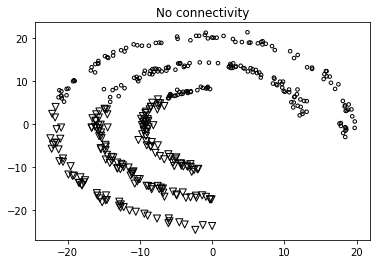
1. Hierarchical clustering refers to a set of clustering algorithms that creates tree-like clusters by consecutively splitting or merging them, and they are represented using a tree.
2. Hierarchical clustering algorithms can be either bottom-up or top-down. Now, what does this mean?
3. In bottom-up algorithms, each data point is treated as a separate cluster
   with a single object. These clusters are then successively merged until all the clusters are merged into a single giant cluster. This is called agglomerative clustering.
4. On the other hand, top-down algorithms start with a giant cluster and successively split these clusters until individual data points are reached. This is called a divisive algorithm.

In hierarchical clustering, we construct clusters by partitioning the instances recursively using a top-down or bottom-up fashion. We can divide these methods as follows:

1. Agglomerative algorithm (bottom-up): Here, we obtain the solution from individual statistical units. At each iteration, we aggregate the most closely- related statistical units and the procedure ends when a single cluster is formed.
2. Divisive algorithm (top-down): Here, all units are in the same class and the unit that is not similar to others is added to a new cluster for each subsequent iteration.

a) Both methods result in a dendrogram.

b) This represents a nested group of objects and the similarity levels at which the groups change.

c) By cutting the dendrogram at the desired similarity level, we can get a clustering of data objects.

d) The merging or division of clusters is performed using a similarity measure, which optimizes a criterion.

Let’s see how to group data using agglomerative clustering:

1. Import the necessary packages:

import numpy as np
import matplotlib.pyplot as plt
from sklearn.cluster import AgglomerativeClustering
from sklearn.neighbors import kneighbors_graph

2. Let’s define the function that we need to perform agglomerative clustering:

def perform_clustering(X, connectivity, title, num_clusters=3, linkage='ward'):
plt.figure()
model = AgglomerativeClustering(linkage=linkage,
connectivity=connectivity, n_clusters=num_clusters)
model.fit(X)

3. Let’s extract the labels and specify the shapes of the markers for the graph:

    #extract labels
labels = model.labels_
# specify marker shapes for different clusters
markers = '.vx'

4. Iterate through the data points and plot them accordingly using different
markers:

    for i, marker in zip(range(num_clusters), markers):
# plot the points belong to the current cluster
plt.scatter(X[labels==i, 0], X[labels==i, 1], s=50,
marker=marker, color='k', facecolors='none')
plt.title(title)

5.In order to demonstrate the advantage of agglomerative clustering, we need to run it on data points that are linked spatially but also located close to each other in space. We want the linked data points to belong to the same cluster, as opposed to data points that are just spatially close to each other. Let’s, now define a function to get a set of data points on a spiral:

def get_spiral(t, noise_amplitude=0.5):
r = t
x = r * np.cos(t)
y = r * np.sin(t)
return add_noise(x, y, noise_amplitude)

6. In the previous function, we added some noise to the curve because it adds some uncertainty. Let’s define this function:

def add_noise(x, y, amplitude):
X = np.concatenate((x, y))
X += amplitude * np.random.randn(2, X.shape[1])
return X.T

7. Now let’s define another function to get datapoints located on a rose curve:

def get_rose(t, noise_amplitude=0.02):
# Equation for "rose" (or rhodonea curve); if k is odd, then
# the curve will have k petals, else it will have 2k petals
k = 5
r = np.cos(k*t) + 0.25
x = r * np.cos(t)
y = r * np.sin(t)
return add_noise(x, y, noise_amplitude)

8. Just to add more variety, let’s also define a hypotrochoid function:

def get_hypotrochoid(t, noise_amplitude=0):
a, b, h = 10.0, 2.0, 4.0
x = (a - b) * np.cos(t) + h * np.cos((a - b) / b * t)
y = (a - b) * np.sin(t) - h * np.sin((a - b) / b * t)
return add_noise(x, y, 0)

9. We are now ready to define the main function:

if __name__=='__main__':
# Generate sample data
n_samples = 500
np.random.seed(2)
t = 2.5 * np.pi * (1 + 2 * np.random.rand(1, n_samples))
X = get_spiral(t)
# No connectivity
connectivity = None
perform_clustering(X, connectivity, 'No connectivity')# Create K-Neighbors graph
connectivity = kneighbors_graph(X, 10, include_self=False)
perform_clustering(X, connectivity, 'K-Neighbors connectivity')
plt.show()