
What is PDF really?
So far, we were looking and looking at the plots of NDs but we did not ask what function generates these plots. To answer this, you need to understand what continuous probability distributions are.
According to descriptive statistics, there are two types of data: discrete and continuous. Any data that is recorded by counting is discrete (integer values) such as the results of test scores, number of apples you eat per day, how many times you stop at a red light, etc. Contrastingly, continuous data is any data that is recorded by measuring such as height, weight, distance, etc. Time itself is also considered as continuous data.
One defining aspect of continuous data is that the same data can be represented in different units of measurement. For example, distance can be measured in miles, kilometers, meters, centimeters, millimeters and the list continues. No matter how small, a smaller unit of measurement can be found for continuous data. This also suggests that there can be infinitely many decimal points for a single measurement.
In probability, if a random experiment generates continuous outcomes, it will have a continuous probability distribution. For example, let’s say random variable X stores the amount of rain every day in inches. Now, it is extremely unlikely for the amount of rain to take an integer value because we cannot say that it rained exactly 2 inches today, not a single water molecule more or less. The probability of that happening is so small that we can safely say it is 0.
The same can be true for other values such as 2.1 or 2.0000091 or 2.000000001. The odds of it raining exactly at some amount is always 0. That’s why for continuous distributions we have different functions called Probability Density Functions. If you were reading my recent posts, Probability Mass Functions computed the probability of discrete events such as die rolls, coin flips, or any other Bernoulli trials.
Probability Mass Functions encode the probability of an outcome as height. Here is an example PMF plot of a single die roll:
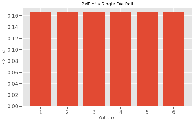
As you see, the height of each bar represents the probability of a single outcome like 1, 3, or 5. They are all at the same height because a die roll has a discrete uniform distribution.
Now, Probability Mass functions use an area to represent a certain probability. Before I explain why think about what would happen if they also encoded probability in height. As I said, there is such a small probability for continuous data to take a certain value that the heights would all go down to 0 like this:

Remember the most favorite formula of statisticians?
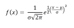
That is the formula for the Probability Density Function of a normal distribution. On its own, it cannot do much. For an ND with a known mean and standard deviation, you can input any x value into the function. It outputs the height of the curve at that point on the XAxis. Notice I am not saying the probability, just the height of the curve. As I said, for continuous distributions area represents a certain probability. Well, a thin line on a plot does not have an area so we need to reframe our initial question.
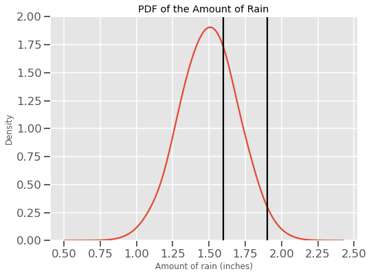
For our random experiment of observing the amount of rain every day, we will stop asking questions like what is the probability of raining 3 inches or 2.5 inches because the answer would always be 0. Instead, we now ask what is the probability of it raining between 1.6 and 1.9 inches. This would be equal to asking what is the area under the curve between these two lines:
For those who did their homework on calculus, it is computed using this integral formula:
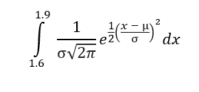
Wait, wait! Don’t go yet. We won’t compute this here by hand or even using code. Later I will show you a much easier way of computing this.
The above formula yields some number between 0 and 1 as the probability of it raining between 1.6 and 1.9 inches. Now, an obvious question is what do we interpret from the YAxis since it does not give the probability. Well, I am in no way qualified to answer this question, so I suggest you read this thread from StackExchange and watch this awesome video by 3Blue3Brown.
Next, we will talk about the Cumulative Distribution function which provides us with a better tool to compute probabilities under areas and maybe an improved visual of NDs.