Code
Read about KNN…
First of all import all the useful libraries which are needed in program.
import math
import numpy as np
import matplotlib.pyplot as plt
import operator
import random
import pandas as pd
For working with arrays, numpy is used. Also matplotlib is a library that is used to plot graphs. Similar to numpy, pandas provides high-performance, easy to use structures and data analysis tools.
After importing libraries, second step is to load the dataset. You can find the dataset which I have used here.
#load train data of respective class
loaddata_train1=np.loadtxt('.../group4/class1_train.txt')
loaddata_train2=np.loadtxt('.../group4/class2_train.txt')#load test data of respective class
loaddata_test1=np.loadtxt('.../group4/class1_test.txt')
loaddata_test2=np.loadtxt('.../group4/class2_test.txt')#concatenate train and test data of different classes in one variable with axis = 0 (row wise)
loaddata_train=np.concatenate((loaddata_train1, loaddata_train2), axis=0)
loaddata_test=np.concatenate((loaddata_test1, loaddata_test2), axis=0)
After loading the data, it’s time to label the data as our original data is unlabeled
#label the data - class1 as 1 and class2 = -1
label1=np.ones((loaddata_train1.shape[0], 1))
label2=np.ones((loaddata_train2.shape[0], 1)) * -1
r1=np.append(label1, loaddata_train1, axis=1)
r2=np.append(label2, loaddata_train2, axis=1)
#concatenate whole train data
train_data=np.concatenate((r1,r2))
Similarly for test data..
#label the data - class1 as 1 and class2 = -1
label3=np.ones((loaddata_test1.shape[0], 1))
label4=np.ones((loaddata_test2.shape[0], 1)) * -1
r3=np.append(label3, loaddata_test1, axis=1)
r4=np.append(label4, loaddata_test2, axis=1)
#concatenate whole test data
test_data=np.concatenate((r3,r4))
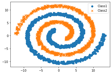
Scatter plot of the dataset. Library used for plotting purpose is matplotlib. We use marker ‘o’ for class1 and marker ‘x’ for class2.
plt.scatter(loaddata_train1[:,0], loaddata_train1[:,1], marker='o', label='Class1')
plt.scatter(loaddata_train2[:,0], loaddata_train2[:,1], marker='x', label='Class2')
plt.legend()
plt.show()
Now according to the algorithm, calculate euclidean distance between every test data point with each train data point.
def euclideanDistance(instance1, instance2, length):
distance = 0
for x in range(length):
distance += pow((float(instance1[x]) - float(instance2[x])), 2)
return math.sqrt(distance)
After calculating euclidean distance, next step is to find out the neighbor, top k values. It is preferred to use odd value of k because it will be easier to find out class label as in even, there may be equal chances of getting same class label.
def getKNeighbors(train_data, testInstance, k):
distances = []
length = len(testInstance)-1
for x in range(len(train_data)):
dist = euclideanDistance(testInstance, train_data[x], length)
distances.append((train_data[x], dist))
distances.sort(key=operator.itemgetter(1))
#     print(distances)
neighbors = []
for x in range(k):
neighbors.append(distances[x][0])
return neighbors
It’s time to get the responses or results from the neighbors we got from the above function.
def getResponse(neighbors):
classVotes = {} #empty dictionary to collect class votes
for x in range(len(neighbors)):
response = neighbors[x][0]
if response in classVotes:
classVotes[response] += 1
else:
classVotes[response] = 1
sortedVotes = sorted(classVotes.items(), key=operator.itemgetter(1), reverse=True)
#print(response)
return sortedVotes[0][0]
After everything is done, define main() function for further and final processing the code.
def main():
l00 = 0
l01 = 0
l10 = 0
l11 = 0
#split = 0.70
print ('Train: ' + repr(len(train_data)))
print ('Test: ' + repr(len(test_data)))
#generate predictions
#predictions = []
k = input("Enter value of k: ")
k = int(k)
list_pred = []
list_act = []
for x in range(len(test_data)):
neighbors = getKNeighbors(train_data, test_data[x], k)
result = getResponse(neighbors)
#predictions.append(result)
list_pred.append(result)
list_act.append(test_data[x][0])
for i in range(0, len(test_data)):
x = list_pred[0]
y = list_act[0]
if int(list_pred[i]) == -1 and int(list_act[i]) == -1:
l00 += 1
elif int(list_pred[i]) == -1 and int(list_act[i]) == 1:
l01 += 1
elif int(list_pred[i]) == 1 and int(list_act[i]) == -1:
l10 += 1
elif int(list_pred[i]) == 1 and int(list_act[i]) == 1:
l11 += 1
i+=1a = np.array([[l00, l01],
[l10, l11]])
print('Confusion Matrix: ')
print(pd.DataFrame(a, columns = ['class_0', 'class_1'], index = ['class_0', 'class_1']))acc = (l00+l11)*100/(l00+l01+l10+l11)
print('Accuracy: ' + repr(acc) +'%')
main()
Result :
Train: 2447
Test: 977
Enter value of k: 5
Confusion Matrix:
class_0  class_1
class_0      488        0
class_1        0      489
Accuracy: 100.0%
