In this article, I do the week 2 programming exercises of the course Machine Learning at Coursera with NumPy. I avoid using frameworks like PyTorch since they are too powerful in comparison with these exercises.
In general, the workflow of a linear regression problem (with one variable or with multiple variables) is presented in the figure below.
It consists of four steps:
- Load Data: load data from text files,
ex1data1.txtandex1data2.txt. - Define functions: define functions to predict outputs, to compute cost, to normalize features, and to carry out the algorithm gradient descent.
- Prepare Data: add column of ones to variables, do normalize features if needed.
- Training: initialize weights, learning rate, and number of iterations (called epochs) then lauch gradient descent.
I also do some more steps of visualization to figure out the data and result obtained.
In this assignment, you need to predict profits for a food truck.
Suppose you are the CEO of a restaurant franchise and considering different cities for opening a new outlet. The chain already has trucks in various cities and you have data for profits and populations from the cities.
The data set is stored in the file ex1data1.txt and is presented in the figure below. A negative value for profit indicates a loss.
1.1. Load data
DATA_FILE = "w2/ex1data1.txt"
data = np.loadtxt(DATA_FILE, delimiter=",")
data[:5,:]
X = data[:,1]  # population
Y = data[:,2]  # profit
- The numpy method
loadtxt()load data from a text file to numpy array.
1.2. Define functions
def predict(X, w):
Yh = np.matmul(X, w)
return Yhdef cost_fn(X, w, Y):
Yh = predict(X, w)
D = Yh - Y
cost = np.mean(D**2)
return costdef gradient_descent(X, Y, w, lr, epochs):
logs = list()
m = X.shape[0]
for i in range(epochs):
# update weights
Yh = predict(X, w)
w = w - (lr/m)*np.matmul(X.T,(Yh-Y))
# compute cost
cost = cost_fn(X, w, Y)
logs.append(cost)
return w, logs
- The numpy method
matmul()perform a matrix product of two arrays.
1.3. Prepare data
X = np.column_stack((np.ones(X.shape[0]), X))  # add column of ones to X
X[:5,]
- The numpy method
column_stack()stacks a sequence of 1-D or 2-D arrays to a single 2-D arrays.
1.4. Training
w = np.zeros(X.shape[1])  # weights initialization
lr = 1e-2  # learning rate
epochs = 1500  # number of iteration
w, logs = gradient_descent(X, Y, w, lr, epochs)
After 1500 iterations we will obtaine the new weights w
array([-3.63029144, 1.16636235])
The line predicted is shown in the figure below.
And the figure below figures out the variation of cost.
In this assignment, you need to predict the prices of houses.
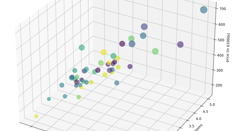
Suppose you are selling your house and you want to know what a good market price would be. The file ex1data2.txt contains a data set of housing prices in Portland, Oregon. The first columns is the size of the house (in square fit), the second column is the number of bedrooms, and the third column is the price of the house.
The figure below presents the data set in 3D space.
There’s only one point that we need to pay attention is house sizes are about 1000 times the number of bedrooms. Therefore, we should perform feature normalization before launching gradient descent so that it converges much more quickly.
Create the function normalize_feature()
def normalize_features(X):
mu = np.mean(X, axis=0)
std = np.std(X, axis=0)
X_norm = (X - mu)/std
return X_norm
Then normalize variables before put them in gradient descent.
X_norm = normalize_features(X)
X_norm = np.column_stack((np.ones(X_norm.shape[0]), X_norm))
The other steps are completely similar to the ones of the assignment above. We don’t need to rewrite functions predict(), cost_fn(), and gradient_descent() since they work well with matrices multi columns.
w = np.zeros(X_norm.shape[1])  # weights initialization
lr = 1e-2  # learning rate
epochs = 400  # number of iterations
w, logs = gradient_descent(X_norm, Y, w, lr, epochs)
After 400 iterations, we have the surface of prediction in the figure below.
You can see that the problem of one variable has the prediction is a line in the surface of inputs and outputs; the problem of two variables has the prediction is a surface in the space of inputs and outputs; the problem of three variables will have the prediction is a space in the 4D space of inputs and outputs; and so on.
From the logs of gradient descent, we also figure out the variation of cost of our model in the figure below.
The code source is at linear regression. If you want to refer to Matlab codes of this programming exercise, they are in the directory w2.