In former articles, we have defined what generalization error is in the context of machine learning, and how to bound it through various inequalities. We also defined overfitting and how it can be remedied by using a validation set. We could avoid the paradox of choosing a size for our validation set by using cross-validation, which turned out to be an unbiased estimator for E_out(N — 1). In this article, we will give some practical examples on which inequalities to use in the case of a validation set and cross-validation.
Example — Validation Set
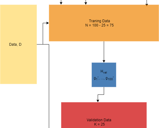
Imagine that we have a dataset, D, with a sample size N = 100. We split our dataset into two parts; a training set with size 75 and a validation set with size 25. We want to evaluate 100 models, which means we have 100 hypothesis sets and find the model with the best performance on our validation set. We will say that all models have d_VC = 10. Then, we want to give an upper bound of our out-of-sample error. Let us first illustrate the process we will go through:
As stated, we have 100 models to evaluate, which gives 100 hypothesis sets. We do not know the dimensions of these hypothesis sets — meaning they can have infinite dimensions. Each hypothesis set is trained on the training data and produces a final hypothesis, g_n-. This indirectly creates a new hypothesis set for our validation data:
We now know the dimensions of our new hypothesis, which is M = 100. We evaluate our hypotheses on the validation set, and we choose the one with the minimum error, E_val(g_m*-). This is our in-sample estimate for E_out(g_m*). We remember that after we have found gm*- then we train the hypothesis on all of the data and give back the model. Since we know the size of our hypothesis set, then we can give an upper bound of our out-of-sample error with:
We remember that our in-sample error, in this case, is E_val(g_m*-), which we use to bound E_out(g_m*-). We do not output gm*-, but gm*. We can though imagine that E_out(g_m*) is equal or smaller than E_out(g_m*-) since we will train our final hypothesis on our whole dataset. All in all, we can say that we have:
An important thing to note is that in this case, N is equal to the size of our validation set! Let us imagine that we choose a confidence level of 95%, i.e., δ = 0.05, and an in-sample error of 0.20. Then we have the following bound:
Imagine instead that we simply trained each model on all the data and selected the function with the minimum in sample error. This would result in a very different process. Let us first illustrate it:
In this case, our hypothesis set is a union of all our 100 hypothesis sets — we do not know how many are in each, so we do not know M. We also do not use a validation set — what we do instead is that each model, Hm, in our hypothesis set produces a final hypothesis, and we choose the one with the minimum error. This is the same as choosing a final hypothesis from the union of all our hypothesis sets — hence we can therefore not say it is a simple, finite hypothesis set. Instead, we need to find the VC dimension of the union of our hypothesis set. All in all, we will have the following bound:
We remember that each hypothesis set has d_VC = 10. We, therefore, need to calculate the VC bound of our hypothesis set first, which can be done with:
Let us say that our final hypothesis still has an in-sample error of 0.20. Then we get the following bound:
We can clearly see that the bound in the former case is tighter.
Example — cross-validation
Imagine that we have a dataset with N samples. You give it to two of your friends. One of them applies 5-fold cross-testing: the data is split into 5 folds and then each time one of the folds is reserved for testing and the remaining four are used to train a prediction model. Each of the 5 folds is used for testing only once. This way your friend obtains 5 prediction models and gives you the one that has achieved the lowest test error. The other friend applies 10-fold cross-testing in the same way and returns you the model with the lowest test error. The two friends work independently of each other. Let h_1∗ be the model produced by the first friend and E_in(h_1*) its test loss and let h_2* be the model produced by the second friend and E_in(h_2*) its test loss. We want to bound the out-of-sample error for each of the hypotheses produced by your friends.
Let us start with friend one and his final hypothesis, which is found through 5-fold cross-validation. We can first visualize the process:
We remember that E_cv is an unbiased estimate of E_out(N — K). We can say that:
We use the inequality for a finite hypothesis set, where M = 5 since our first friend produces 5 hypotheses in total. Our in-sample-error is equal to E_cv. N is still N since all the data has been used in total. Hence, we have the following:
Let us now do the same for the friend who implements 10-fold cross-validation. Then we would have:
Now we have 10 models, so we would get the following bound:
Conclusion
We have now seen some examples of how the different bounds can be used in different scenarios when using either cross-validation or a simple validation set. In the next article, we will see how we can estimate the generalization error in the specific case of using Support Vector Machines.
