Deep learning is also a powerful tool for Biologists
In this entry, I show how to harness deep mutational data and embeddings derived from a protein language model (ESM-1b) to predict if a receptor binding domain (RBD) variant from the COVID-19 Spike protein (S) has an increased affinity towards the human ACE2 receptor. At the end of the article, I also show how to reuse these embeddings for other purposes such as the prediction of antibody escape mutants.
The protein responsible for the binding of COVID-19 to human cells (and thus start the infection) is the spike protein (S) and specifically, it binds the ACE2 receptor with the region known as the receptor binding domain (RBD). Proteins are simply strings composed of an alphabet of 20 letters or amino acids (aa), and in the case of the original Wuhan strain, the spike protein has a length of 1273 aa. Not surprisingly, the strength with which S binds the human ACE2 receptor is a function of the specific sequence of amino acids of the RBD (along with other factors such as the ACE2 sequence, but here I focus only on the RBD).
Formally, what we want to find is a function (f) that maps a specific RBD sequence to a score between 0–1. Where given a threshold t, if f(S) > t, then we predict that a RBD binds stronger to ACE2 than the original variant (Wuhan-Hu-1 strain).
Our training set will consist of a set of mutated sequences of the RBD of S along with their corresponding experimental binding strength to the human ACE2 receptor. This dataset is derived from the paper “Deep Mutational Scanning of SARS-CoV-2 Receptor Binding Domain Reveals Constraints on Folding and ACE2 Binding”. In this paper, Starr et al managed to estimate the binding strength of different RBDs by generating mutants in a high-throughput manner using a yeast-display system. If you go to the Supplemental Information, you will find Table S2 which contains the dataset that we are going to use. The “mutant” column indicates amino acid changes and at which position of S occurred, while “bind_avg” is the experimental affinity defined as Δlog10(KD,app) relative to the Wuhan-Hu-1 strain.
After regenerating the full sequence for each variant of S, I removed all the mutants with nonsense mutations and deleted the corresponding S2 subunit portion of S. Even though all the mutations are directed to the RBD region of S, I left the whole S1 subunit given that long-range interactions are common in proteins. A caveat is that although the classifier is trained with whole S1 sequences, in principle it will not be able to generate reliable predictions for mutations occurring out of the RBD region.
As mentioned in the beginning, the goal is to train a classifier to identify RBD variants that bind tighter to the ACE2 receptor than the one from the Wuhan-Hu-1 strain. Thus, we need a suitable representation of the mutant sequences. Here we are going to use embeddings from a state-of-the-art transformer protein language model (ESM-1b) which you can find here. This transformer was pre-trained by Rives et al in an unsupervised way and it learned to abstract key features of proteins such as secondary and tertiary structure. You can find more details about how it was trained in their paper “Biological structure and function emerge from scaling unsupervised learning to 250 million protein sequences”.
All the protein embeddings extracted from the transformer are fixed vectors with 1280 elements and thus they are ready to be processed by classic classifiers. In this work, I use a random forest (RF) to perform the classification. Below you can see the pipeline of the model.
After generating embeddings for all the RBD mutants, I binarised the experimental affinity. If Δlog10(KD,app)>0, that means that the RBD from S1 has higher affinity than the Wuhan-Hu-1 strain and thus y=1, otherwise y=0. Finally, I partitioned the data into train, validation, and test datasets with proportions 60:20:20.
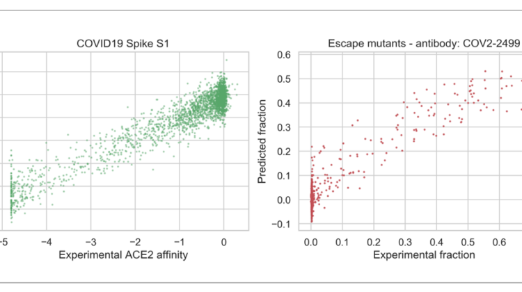
Before proceeding with the random forest, I took a quick look at the training data by means of linear regression. This analysis would give me a glimpse of the potential of the features encoded in the protein embedding to predict the experimental affinity. Importantly, for this analysis I kept the original non-binarised Δlog10(KD,app). As can be seen from the left plot below, there is a good correlation between the experimental and predicted affinities (Pearson r: 0.945, p ~ 0). Interestingly, when I used PCA to collapse the 1280-dimensional embedding into the two main 2 components, the correlation disappears. Thus, this result highlights the importance of equally weighting all the elements of the original embedding to improve the performance of the classifier.
After training a RF with a max depth of 5 and 300 estimators with the train dataset, I visualised a subset of the predictions along with the experimental data. In the graph below, the binarised experimental affinity is plotted in blue along with the predicted scores by the RF in orange. As you can see, the RF is learning to score higher the variants with Δlog10(KD,app)>0. I also plotted as a reference in green the non-binarised experimental affinity (minimum value truncated to -1 for visualisation purposes).
In order to select the best model, I trained the RF with the train dataset and tuned the number of trees (100, 300, 500, 800) and maximum depth (2, 5, 7, 9, 10) hyperparameters. For each model, I then evaluated the performance by calculating the area under the ROC curve using the validation dataset. As seen in the ROC curves below, across all number of trees, a maximum depth of 2 always results in a significantly decreased performance in the validation dataset. For all the other maximum depths, performance seems to be similar.
Plotting the area under the ROC curve for all the models, shows that the model with the highest performance consisted of 500 trees and a maximum depth of 9. Evaluating the performance of the best model with the test dataset outputs an area under the ROC curve of 0.706.
We finally have a working RF model and now we need to decide the threshold at which we consider a spike variant to bind tighter to the ACE2 receptor. Picking the threshold is a trade-off between false negatives and false positives. If we were to deploy a genomic surveillance plan, predicting false negatives can be very costly, thus we want to put more weight on the recall. On the other hand, predicting an excess of false positives can result in unnecessary false alarms which can cause severe disruption. For this example, we are going to pick a threshold of 0.3, which corresponds to a recall of 46.26% at the expense of a false positive rate of 18.94%.
In order to get a better sense of how different thresholds perform in the test set, below you can find a scatterplot of each variant’s RF score, along with their corresponding experimental affinity values. The majority of the variants with Δlog10(KD,app) > 0 are predicted to have a RF score > 0.3. Although you can also see in the lower right part of the plot that some variants with high Δlog10(KD,app) are not classified as positive hits. Another observation is that even though many false positives are found at an RF score > 0.3, they usually have a Δlog10(KD,app) > -1, indicating that maybe the model was picking up features that segregate variants with really bad affinity to ACE2.
I then reused the transformer embeddings to link mutations in the RBD of the Spike protein that escape antibody binding. The data comes from the paper “Complete Mapping of Mutations to the SARS-CoV-2 Spike Receptor-Binding Domain that Escape Antibody Recognition”. In this paper, Greaney et al mapped RBD escape mutations to 10 human monoclonal antibodies and just like with Starr et al, a yeast-display system was used to generate the data. The data can be found in Table S1. Each dot in the plots below represents a different RBD mutation and the x-axis represent the fraction of cell expressing that mutation that fell into the antibody-escape sort bin. As you can see below, the regression models do a decent job at predicting escape fraction (all Pearson r’s > 0.8).
Machine learning and specifically deep learning (DL) has experimented an explosive growth in the last decade and recently it has had breakthroughs in biology (e.g. AlphaFold and the development of protein language models). The goal of this post was to show how these novel developments in DL have the potential to be harnessed for real-world applications such as prediction of the binding strength between a virus and its human receptor or the prediction of escape mutants.