As you can see, the Bisection Method converges to a solution which depends on the tolerance and number of iteration the algorithm performs. There is a dependency between the tolerance and number of iterations. For a particular tolerance we can calculate how many iterations n we need to perform.
Every iteration the algorithm generates a series of intervals [an, bn] which is half of the previous one:
The tolerance ε is the absolute value of the difference between the actual root of the function x and the approximation c.
For the algorithm to converge within an absolute error tolerance (ε), we need to have:
By replacing inequality (3) with equation (1), we get:
Solving inequality (4), we obtain:
We apply the logarithm function to both sides of the inequality (5):
From the above result we can understand that, using the Bisection Method, in order to calculate an approximate root of a function within tolerance ε, the number n of iterations we need to perform is:
For the example presented in the above example our algorithm performed 9 iterations until it found the solution within the imposed tolerance. Let’s apply the above formula to see what is the minimum calculated number of iterations.
The result shown that we need at least 9 iterations (the integer of 9.45) to converge the solution within the predefined tolerance, which is exactly how many iterations our algorithm performed.
So, to summarize zero-order methods these are used back in optimizing the losses in perceptron or multi-perceptrons back during the starting of neural-networks. These are kind of slow as they need more iterations and converge slowly so to overCome this problem scientist adopted first-order methods that we regularly utilize.
First-Order Optimization Algorithms
1. Newtons Raphson Method (for single variable):
The Newton-Raphson method (also known as Newton’s method) is a way to quickly find a good approximation for the root of a real-valued function f(x)=0f(x) = 0f(x)=0. It uses the idea that a continuous and differentiable function can be approximated by a straight line tangent to it.
Basically, it is an iterative algorithm for finding a points where the function is zero (or) zeros of the function. When applied for optimization it gives a procedure for finding minima or maxima of a function.
How it works?
Suppose you need to find the root of a continuous, differentiable function f(x), and you know the root you are looking for is near the point x = x_0. Then Newton’s method tells us that a better approximation for the root is
This process may be repeated as many times as necessary to get the desired accuracy. In general, for any x-value x_n, the next value is given by
Note: the term “near” is used loosely because it does not need a precise definition in this context. However, x_0 should be closer to the root you need than to any other root(if the function has multiple roots).
Geometric Representation
We draw a tangent line to the graph of f(x) at the point x = x_n. This line has slope f¹(x_n) and goes through the point (x_n, f(x_n)). Therefore it has the equation y = f¹(x_n)(x-x_n) + f(x_n). Now , we find the root of this tangent line by setting y = 0 and x = x_n+1 for our new approximation. Solving this equation gives us our new approximation, which is
Numerical Example
In this simple case, we have only minimized a function of a single variable. This is useful to illustrate the concept, however, in real-life scenarios, millions of variables can be present. For neural networks, this is definitely the case. In the next part, we are going to see how this simple algorithm can be generalized for optimizing multidimensional functions!
Newton’s Method(multi-variable method):
Newton’s method is a second order function which means it not only uses first derivative (i.e. gradient) but also the second derivative (i.e. hessian) in the multi-variable case.
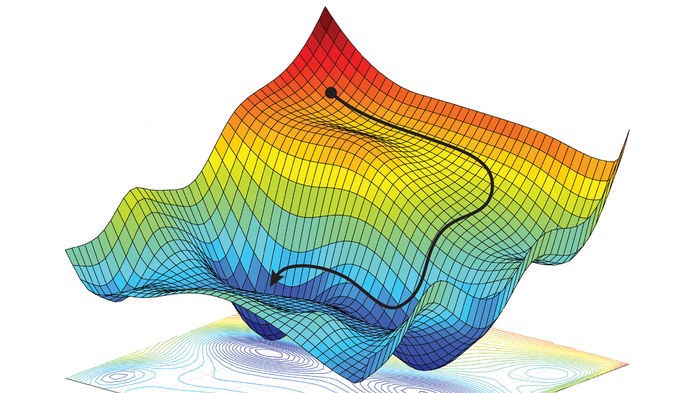
This method gives us a advantage of optimizing our variables in multiple dimensions as there are multiple variables our function in graph doesn’t look like a single quadratic parabola shape it looks like a plane or surface.
how do it max/min the function?
This actually does a second order approximation of function using quadratic/symmetric plane and you minimize that by taking x_t+1 as new minima of function.
Let’s extend this concept to two dimensional
The center point (m) is minima that we want to reach. We start off at some random point x_t which is random in outer plane and estimate its second order derivative and reach its new minima x_t+1
This process is iterative and it reaches to minimum to m.So our idea is to make a 2nd order approx and min that
Let f:R^n ==> r be (suff) smooth , then to make a second order approximation we make it a polynomial approximation to the function using taylor’s theorm.
Taylor’s theorm tells us that F can be approximated so if we have some point at “a” and we want to look at points “x” which are near ‘a’ then
Let’s minimize the quadratic approx. of f by taking gradients
Here the hessain may (or) may not be invertible which is one sort of coviot here. If X = a-H¹g that is our critical point and to check that if it is min, we need to see that it is least possible semi definite & to do that we need to take its 2nd derivative.
So these are the first-order optimization algorithms that are used in the process of finding the gradients in the back-propagation. To be precise this newton’s method is used in gradient descent to calculate gradients. And there are some other extra space or variables added to gradient descent to get the remaining optimization algorithms in keras.
Final Note:
To conclude this article I would say that not just knowing how to code these optimizers in our code, its always exciting to know the math behind these algorithms and is always important to know these algorithms that run behind the wall of api calls.
Thanks for reading the article and may in the upcoming article i’ll give you guys the intuition of the optimization algorithms in keras.