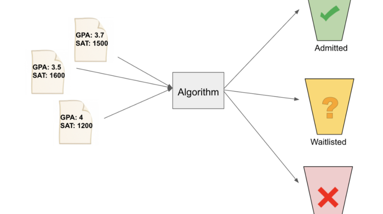
Logic behind Softmax regression
Ultimately, the algorithm is going to find a boundary line for each class. Something like the image below (but not actually the image below):
Note: we as humans can easily eyeball the chart and categorize Sarah as waitlisted, but let’s let the machine figure it out via machine learning yeah?
Just like in linear and logistic regressions, we want the output of the model to be as close as possible to the actual label. Any difference between the label and output will contribute to the “loss” of the function. The model learns via minimizing this loss.
There are 3 classes in this example, so the label of our data, along with the output, are going to be vectors of 3 values. Each value associated with an admission status.
If the label is such that:
admitted = [1, 0, 0]
waitlisted = [0, 1, 0]
rejected = [0, 0, 1]
then the output vector will mean:
[probability of being admitted,
probability of being waitlisted,
probability of being rejected]
Thus, in softmax regression, we want to find a probability distribution over all the classes for each datapoint.
We use the softmax function to find this probability distribution:
Why softmax function? I think this functions is best explained through an example. Let’s look at the example:
GPA = 4.5, exam score = 90, and status = admitted.
When we train a model, we initialize the model with a guessed set of parameters — theta. Through gradient descent, we optimize those parameters. Because we have 3 classes (admitted, rejected, and waitlisted), we’ll need three sets of parameters. Each class will have its own set of parameters.
Let’s have theta be of the shape:
[bias, weight of GPA, weight of exam score]
Let’s initialize thetas to be:
theta_admitted = [-250, 40, 1]
theta_waitlisted = [-220, 40, 1]
theta_rejected = [-220, 40, 1]
Why those values?
Remember that a line is y = mx + b? The line given by the initial thetas would be:
admitted:
-250 + 40x + y = 0
y = -40x + 250waitlisted:
-220 + 40x + y = 0
y = -40x + 220rejected:
-220 + 40x + y = 0
y = -40x + 220
If I just eyeball the data, I can see that the line that separates “admitted” from the rest has y-intercept around 250 and slope around -40.
Note: It’s a start, but these parameters are actually never going to work. First, the parameters for waitlisted and rejected are the same, so the parameters will always return the same probability for waitlisted and rejected regardless of what the input is. Second, only the bias differ, and rejected and waitlisted have a bigger bias than admitted (-220 > -250). Therefore, regardless of what the input is, these parameters will return 0 for admitted and 0.5 for the other two.
But it’s okay to start with bad parameters, the model with fix it!
Let’s visualize what the softmax function is doing.
What happens when we run our datapoint through the softmax equation? Again, our datapoint is: GPA = 4.5, exam score = 90.
First, we find the dot product of the parameters and datapoint:
Then, we exponentiate that value to get rid of any potential negative dot products:
Lastly, we normalize it to get a probability distribution:
Because our initial set of parameters are not good, the model output 0.5 for rejected and 0.5 for waitlisted even though the label is admitted.
Essentially, the softmax function normalizes an input vector, into a probability distribution. In the example we just walked through, the input vector is comprised of the dot product of each class’ parameters and the training data (i.e. [20, 50, 50]). The output is the probability distribution [0, 0.5, 0.5].
The machine learning algorithm will adjust the bias, weight of GPA, and weight of exam score so that the input vector will produce an output distribution that closely match the input label.
What we really want is our model to output something like:
So, let’s change the parameters for all three classes to get better accuracy.
One way to do this is by gradient descent.
Gradient descent works by minimizing the loss function. In linear regression, that loss is the sum of squared errors. In softmax regression, that loss is the distance between the label and the output probability distribution.
This loss is called the cross entropy. The formula for cross entropy is:
The inner 1{y=k} evaluates to 1 if the datapoint x^i belongs to class k. 1{y=k} evaluates to 0 if datapoint x^i does not belong to class k.
Essentially, this function is measuring how similar the label and output vectors are. Here’s a good blog post that goes into detail about this equation.
The total cross entropy, or loss, will be the sum of all the cross entropies normalized over number of training examples.
We take the derivative with respect to theta on this loss in order to do gradient descent.
The new parameters for class k after each iteration is:
Again, 1{y=k} will be 1 if x^i belongs to class k, and 0 if x^i does not belong to class k.
We use this formula to calculate new thetas for each class.
Now, let’s implement the algorithm to arrive at optimal parameters theta.
