For this article, I’m assuming that you know the basics of the Perceptron algorithm.
Linear models often serve the purpose of modeling data well, but sometimes it is not enough. To be more concrete, I will introduce the topic with an example:
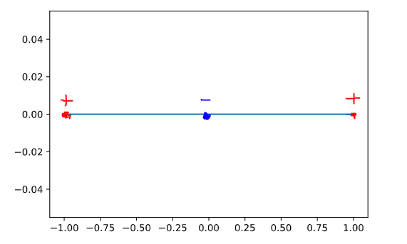
Suppose that we are dealing with a simple feature vector that lives on the real line. in other words:
For the sake of simplicity, let’s consider 3 data points described as follows:
If you try to implement a linear classifier in these feature vectors, you will fail, because no linear classifier can separate this.
Well, to remedy this issue, high-order feature vectors come to play. The idea is simple yet elegant: If we make a function that allows us to expand the information about features in a high dimension space and this space, we use what we already know about linear models?
What do I mean by this? Let’s be more precise:
Pick the same example that I gave before and let’s define a function that can transform this feature vector in a high dimension space:
And now, let’s see if we can separate these feature vectors in the transformed space:
Now we can draw a set of possible decision boundaries(dashed lines) that can separate those examples. The first time that I saw that it was a great wow!
Well, that’s awesome, but if our feature vector lives in a more complex space? I have good and bad news: The good is that the same process can be done to more complex feature vectors, in addition to that we can use other transformations that are not x²(t). Let me give an example: Suppose that
Such that
Now, if we construct a transformed feature vector with a 2-degree polynomial, we have:
You can see that using only a 2-degree polynomial, we get much more features than we used to have. In this case, we have 5150. To be more specific, when we have “n” terms and we get a “p” order polynomial, the total number of terms that our transformed feature vector will have can be calculated as follows:
To exercise a little bit, let’s change the degree of the polynomial to 3 and see what happens to the number of terms:
Wow! it scaled quickly. When I saw this, I thought: here comes the bottleneck. Can we do better? The answer is YES!
This text so far motivates what comes next: Kernel Functions.
What are Kernel functions?
Kernel functions are functions that map “n” dimension vector to “m” dimension vectors using dot products between two vectors.
The soul of kernel functions is the following: We choose a well-behaved kernel function (simple and easy to compute dot product) and we do not define explicitly what feature transformation we are using, but instead, we define in terms of kernels.
Ok… but why is that useful? The answer is: We can emulate an infinite degree polynomial (and get this level of complexity added to the model) without the need to compute all those terms that we saw without using kernel functions. What??? Yes. you heard just right. Let’s see how the original Perceptron work, and how we can modify the original algorithm to work with kernels.
To modify this algorithm, we will use
And get this form:
Ok… if we think about it for a second we realize that the final theta will be in this form:
Where the alphas are the number of mistakes that the “j” data point did. If we multiply both sides by the feature transformation applied on x_i, we get:
And now the magic begins: this equation is the same as…
Ok kernels… now you got my attention!
So… if we modify again the algorithm to work in terms of alphas and not thetas, we get:
Please note that the update of alphas is the same as update thetas. (try to prove it.) Hint: Expand this equation.
Ok… now we got an algorithm in terms of alphas and kernel functions that can handle the Perceptron algorithm, but we still need to select some convenient kernel function to work on. Let’s see an example that demonstrates the power of kernels:
Let’s define this kernel known as Radial Basis Kernel.
If you recall Fourier, you might remember that exponential functions can be described by infinite degree polynomials, and by invoking this kernel, we are implicitly adding an arbitrary powerful model to the table, and the best part is: We did not even define what transformation function did we use, and this doesn’t matter at all, all we need is this nice behaved kernel. Awesome!!
To summarize the ideas, with this methodology we solved a non-linear problem in the original space (getting a non-linear decision boundary), by using a linear method on the transformed space indirectly with the smart usage of kernel functions.
Some caveats:
- We have some rules to compose new kernel functions:
2. There are several other kernel functions to use.
Hope you enjoyed this subject as much as I do =)
