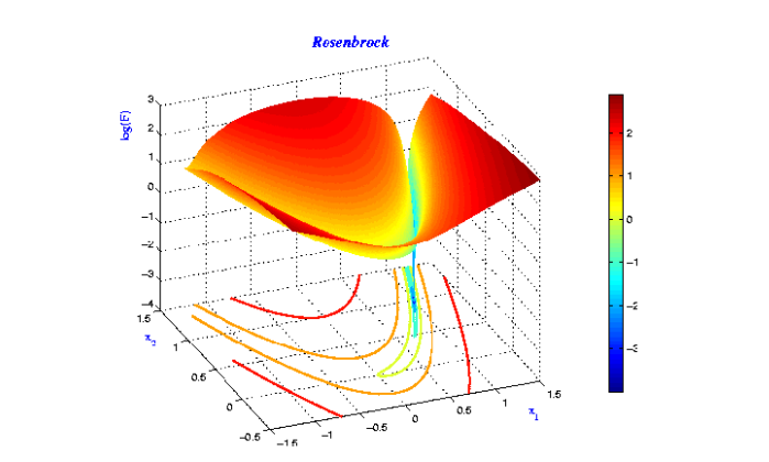
- Model is a function approximated by a neural network after training.
- To determine how good a fit is, loss function is used.
- When the model and loss function are combined we get an optimization problem.
- Objective function is a loss function in which the model is plugged in i.e., it is parameterized by model parameters.
- Optimization involves minimizing an objective/cost function with respect to model parameters.
- Gradient descent is used to optimize neural networks.
- A gradient is obtained by differentiating(calculus) the objective function with respect to the parameters.
- Minimization means to update the parameters in the opposite direction of the gradient.
- Learning rate is the size of the step taken to reach a global/local minima.
- SGD iteratively updates the gradients by calculating it for one example at a time.
- It is fast and can be used for online learning.
- In mini-batch gradient descent, instead of iterating over each examples, the gradient is calculated on a batch size of n.
- Frequent updates with high variance result in high fluctuations.
- Fluctuations result in jumping from one local minima to the other complicating convergence.
- But, it is shown that when the learning rate is decreased slowly, it converges to local or global minima.
- Usually when SGD is mentioned, it means SGD using mini-batches.
- It is difficult to choose a proper learning rate
- Learning rate can be reduced according to a pre-defined schedule or depending upon when the change in the objective between epochs falls below a threshold. These schedules and thresholds have to be defined in advance and wont adapt to dataset’s characteristics.
- The same learning rate is applied to all parameters.
- Escaping from suboptimal local minima and saddle points traps.
- Accelerates SGD in the appropriate direction and also reduces oscillations.
- NAG is is better than Momentum.
- The anticipatory NAG update prevents us from going too fast and results in increased responsiveness.
- Updates are adapted to the slope of the error function and results in more speed than SGD.
- Has per parameter learning rate and uses low learning rates for high frequency features and high learning rates for low frequency features.
- Suitable for dealing with sparse data.
- No manual tuning of learning rates is required.
- Default learning rate is 0.01
- Learning rate of this algorithm shrinks.
Note: if the learning rate is infinitesimally small, the algorithm cannot learn.
- This is an extension of Adagrad that seeks to reduce its aggressive, diminishing learning rate.
- No need to set a default learning rate.
- Solves Adagrad’s radically diminishing learning rates.
- Suggested default values: Momentum, γ = 0.9, learning rate, η = 0.001.
- Adam is another method that computes adaptive learning rates for each parameter.
- Adam can be viewed as a combination of RMSprop and momentum.
- Default values are 0.9 for β1, 0.999 for β2, and 10−8 for ϵ.
- Updates are more stable as infinity norm is used.
- Default values are η=0.002, β1=0.9, and β2=0.999.
- Nadam combines Adam and NAG.
- Adaptive learning rate methods in some cases are outperformed by SGD with momentum.
- The solution of Adaptive learning rate methods has the following disadvantages: a) Diminishes the influence of large and informative gradients which leads to poor convergence. b) Results in short-term memory of the gradients which becomes an obstacle in other scenarios.
- Because of the above reasons, the following algorithms have poor generalization behaviour: Adadelta, RMSprop, Adam, AdaMax, and Nadam
- AMSGrad results in a non-increasing step size, which results in good generalization behavior.
