A Machine Learning Approach to the NYC Property Market
New York City is one of the flagship metropolises of the USA, and therefore, by extension, one of the most influential cities in the world. The state of New York is the third largest in America behind California and Texas, and if it were its own nation, it would be the 10th largest economy on the planet. It has a population of almost 8.5 million, the most populous in the United States. It is by all standards, an international city, with peoples and cultures from across the world.
The property market in NYC has long been one of the most expensive in the world. It is the tenth most expensive in the world, behind cities like Hong Kong, Munich, Los Angeles and others. According to Redfin.com, in October 2020, the median price listing for homes was $850,000 , and the average sale price was $670,000. Property prices can be affected by a number of factors, including square footage, location, type of house, surrounding amenities, crime rates, proximity to schools and offices, and much more.
This report was written as part of a Capstone Project for the IBM Coursera Data Science program.
The best decisions are made with evidence, logic and reason. A machine learning model can provide one layer of evidence to a firm or investor when making decisions, especially with an industry such as the property market. A buyer or seller needs all the information available to them, in order to make the best possible decision. Machine Learning models are important and can help because they show relationships and insights in previously obtuse data, or help to quantify relationships that have been qualitatively verified.
The central problem of this report will be identifying relationships between the following variables in property:
- Number of reported crimes within a roughly 100m (0.0015°) radius in a given 12 month period
- Number of venues within a 200m radius (Redacted due to billing errors)
- Total square footage
The aim will be to predict the price of a property unit using these characteristics. This concept would be beneficial to buyers and sellers in the property market, whether they be homeowners or investors, who can use models to approximate what their property is worth.
One detail to keep in mind is that the property prices can fluctuate over time, completely independent of the physical properties of the property itself. If you were to leave an apartment alone for a decade, its price would likely oscillate greatly with the economy, changing trends and fashions and many other factors. It is for this reason a dataset for sales within a relatively short time period was chosen, as it is unlikely for these external factors to vary greatly in 12 months, especially in the context of Pre-COVID New York.
One point that would be pertinent to note, there are a plethora of factors that affect property prices, and the variables to be used in this project are by no means an exhaustive list. Most of the variables would be out of scope of this project, and the objective is to focus on a few. As such, any predictions will have a certain amount of error associated, as the real-world sales used for the predictions have a potentially infinite number of variables associated with them which a simple model could not possibly control for.
Given that a model is only as good as the data you feed into it, finding a well curated, and complete dataset is vital to the success of any investigation. Hence, rather than form a question, and find a dataset to answer it, I decided to do the opposite. I found data and formed my business problem around it.
I scoured Kaggle, and located a dataset from the City of New York, named “ NYC Property Sales, a year’s worth of properties sold on the NYC real estate market ”. According to the description, it is “ a concatenated and slightly cleaned-up version of the New York City Department of Finance’s Rolling Sales dataset ”. It has a record of every building or building unit sold in NYC from 2016–2017.
Another dataset I found on Kaggle was the “ New York City Crimes ” dataset, described as “ 2014–2015 Crimes reported in all 5 boroughs of New York City ”. Even though the dates for the two datasets don’t match up, the crime rates in New York between 2014 and 2016 are sufficiently similar that a comparison can be drawn. Moreover, even if crime overall decreases, the proportion of crime in each area of the city, with respect to one another, is going to remain constant, as wealthy and poor areas are likely to remain how they are in such a short span of time.
Finally, the Foursquare API will be used to query venue data from FourSquare, in order to get information such as the most popular venues in a certain area, its popularity, and so on. I will be using longitude and latitude values derived from property addresses to query the number of venues in the near vicinity. This information will get queried, and will get wrangled, cleaned, and assimilated into a dataframe with the rest of the data.
(Unfortunately I will not be able to query this data due to billing errors with the FourSquare API and hence will have to abandon this data source)
The NYC property sales dataset has 22 columns, with a variety of headers, from ‘ Date Built ’, to ‘ Tax Class at Time of Sale ’. However, there are only a few columns that pertain to my investigation:
- LAND SQUARE FEET
- GROSS SQUARE FEET
- SALE PRICE
- ADDRESS (To be used to retrieve results for other queries)
All extra columns will be dropped
The dataset on crime contains 22 columns, with many details about incidents such as incident date, offense description, location, and so on. However, for my purposes, I am not analysing the crimes themselves, Ijust need to know how many of them occurred within a given radius. Hence, I only require columns relating to the location of offenses, as well as an attribute to serve as a primary key, such as perhaps the ‘ CMPLNT_NUM ‘ column, which is a randomly generated ID for each complaint. Hence, I will be using the following columns :
- CMPLNT_NUM
- Latitude
- Longitude
All extra columns will be dropped
My final source of data will be FourSquare, where I will be querying data from the FourSquare API. For my purposes, I will be querying the number of venues within a one hundred metre radius. This information will not be queried directly, I will need to query the venues and then separately determine the number of venues that were queried. (Unfortunately I was not be able to query this data due to billing errors with the FourSquare API and hence had to abandon this data source)
I will be using the location of the properties as input to the query, the results of which will be nearby venues.
I used IBM’s inbuilt tools to import the two CSV files, nyc_rolling_sales and NYPD_Complaint_Data_Historic, and proceeded to clean it.
Firstly, the sales data. I read it to dataframe and removed the columns that I wasn’t going to be using. I had already noticed on preliminary analysis that null values in the dataset were represented by a ‘-’ symbol, so I had to replace all instances of that character with a numeric ‘0’. Then I converted the three columns with numeric values that I was interested in (namely : Sale price, Gross square footage and Land square footage), from string form into integer form. This is to allow my model in the future to be able to receive it as input.
One point to note is regarding the square footage columns. There are a number of rows with either of the ‘ Land ’ or ‘ Gross ’ square footage columns empty, or, in some cases, both. Unfortunately, I do not have real estate experience, so I am unable to tell if these are correct or indeed omissions. Hence, in order to simplify the process, I created a column named ‘ Total Area ‘ , which is a sum of the land areas and gross areas for each sale. I then filtered out all the properties with a 0 total area, and dropped the original Land and Gross columns.
After this I had to retrieve the exact geographical locations of each of the sales, so that the nearby crimes and venues could be calculated from it. This was done through the geolocator library, and was very hardware intensive, as I had to pass the address, retrieve the longitude and latitude, and append it to the list, for each and every address for over 26,000 properties. The execution took several hours, and I had to drop the rows in which the GeoLocator function could not retrieve the location.
Next, the crime dataset had to be taken in and cleaned. Fortunately, I had drastically fewer columns to be taken in and cleaned. I read the dataset into a dataframe and dropped all unnecessary columns. I then plotted distributions of the Longitudes and Latitudes to make sure that they fell within the proper ranges.
The crime data was much easier to clean and verify, because unlike the sales data set, I didn’t require details, I simply needed to verify that the crime occurred and that a location was given.
After this, I had to query the FourSquare API to get the number of venues near every property in the dataset. I did this with a loop, and created a list of the number of venues within 200 meters of each property, which I then promptly combined with the sales data, which now had the address, total square footage, sale price, longitude, latitude, and number of venues within 200 meters as fields. (Unfortunately I was not be able to query this data due to billing errors with the FourSquare API and hence had to abandon this data source)
The final step in cleaning my data was to retrieve the number of crimes that occurred within 100 meters of every property sale. I did this by calculating the rough decimal degrees equivalent of 100 meters (0.0015°), and searched for every complaint that occurred within that range, for both longitude and latitude. This creates a square of area, with the property as the center, and every complaint that occurred in that area is tallied, and assigned to that property. This was the final step in cleaning, and I now have my final dataframe to perform exploratory data analysis upon, and eventually, modelling and accuracy testing.
For a univariate analysis, I plotted the distribution of each variable and tried to identify and remove outliers that could potentially skew results and bias models. The goal was to get distributions that resembled normality.
From this I can determine that the vast majority of area values lie between 0 and 200,000, and so I plotted again and again, refining the maximum area until the distribution approached something close to a normal distribution. This was to remove outliers and prevent the large values from skewing the model. I set the maximum total area to 12,000 square feet, and got this plot :
Next I plotted the distribution of crimes within roughly 100m of every property :
This shows us that the distribution of crime data was close to normal, with a number of outliers slightly skewing the results, so I filtered the dataset to remove outliers by setting the maximum number of crimes to 25, and obtained the following plot, looking much closer to a normal distribution :
At this point, I noticed that there were some values listed as ‘0’ in the ‘ Sale Price ‘ column. The description of the data set mentioned that sales where the price was some ridiculously small value such as $0, or $1, was simply a nominal value that was paid solely to facilitate the passing on of property from one person to another, often in the form of parents passing property to children, and so on. I decided to investigate this, so I plotted the distribution of prices :
The graph showed that the vast majority of points lay within $0 and $500,000,000, with only a few outliers, presumably for large buildings worth hundreds of millions of dollars. The frequency of sale price started at a local maximum at $0, presumably for the people bequeathing their homes. It then trends downwards, before rising dramatically. To get more information, I searched for all properties in the state of New York, and sorted for the cheapest properties. The lowest I could find was an agricultural lot for $19,000.
From this preliminary analysis, and given the volume of data at my disposal, I have decided to keep the minimum reasonable sale price at 15,000 to allow for any possible cheaper sales that may have occurred in the past, as well to mitigate the possible effects of inflation. I also decided to make the maximum sale price 2,000,000, because the vast majority (over 90%) of my data after the minimum price restriction was still present after executing a $2,000,000 maximum sale price. The massive multi-billion dollar sale prices, if left in, could potentially have drastically biased the results. The dataset after restrictions applied is now over 26,000 rows long at the end of cleaning.
Finally I used the .describe() method to get a basic statistical inference of the dataset as a whole:
For multivariate analysis, I plotted my two input variables against my target variables, visually assessed the correlation and calculated the Pearson correlation coefficient for each. The Pearson correlation coefficient is the covariance of two variables divided by the product of their standard deviations.
First, I plotted total area against sale price :
As you can see, there are a massive number of data points, and they are very much spread out. The calculated Pearson correlation coefficient is 0.2995808021778173. This shows that total area and price have a positive correlation, however there are still a number of other factors that determine the sale price, and total area is just one of the factors. However, it would make sense that, in the long run, a higher total area means a higher sale price.
Next I plotted nearby crimes against sale price :
Here I see that in general, the sale price goes down as crime rates go up, however, as crime rates go up, the distribution (black line on top of the bars) of the prices also goes up. The Pearson correlation coefficient of nearby crimes against sale price is quite low at : -0.1515061470522369. It shows that there is a negative correlation between the two, which would be something that the average person would be able to guess, however that the correlation is loose at best.
Finally, to conclude my exploratory data analysis, I plotted all three variables together to try and better visualize any relationship. First I plotted them together, with sale price as on the third, z axis :
In order to prevent the plot from being cluttered, I took a sample of 1000 random property sales, and plotted them. It is faint, but it is possible to observe that as nearby crimes tend to zero, and total area tends to twelve thousand, that property prices do go up. However, the 2D representation of a 3D graph leaves much to be desired, so I plotted them against each other on a 2D plane, with color as the third axis :
It is faint, but I see that the color gets somewhat darker as you approach the top left, at which the total area goes up and nearby crimes go down.
There are a variety of models that I can use. Anywhere from K-means to logistic regression, however, for my purposes, I must take a look at my input and target variables. My target variable is continuous, I am trying to predict the price of a property, which can take any value in a range. Additionally, my input variables are also continuous : total area and nearby crimes. Hence, I decided to use Multiple Linear Regression.
Multiple linear regression uses multiple variables, in my case : total area and nearby crimes. These are combined with coefficients and an intercept to make an equation in the following configuration :
The coefficients b in the above graphic are those which need to be decided by my model. There are a number of specific algorithms for this, but in general, I need to minimise error. There are many ways of estimating error, but one is MSE, or mean squared error, given by the following formula :
In any case, my model iterates through a number of possible values of b or the coefficients, and calculates the error for this. Then, it has to find the point at which error is minimised. There are a number of algorithms for the following, such as gradient descent, which works by taking steps down or up a function to locate the minimum.
Once this minimum has been found, the corresponding coefficients are then used to predict the target variable based on the given inputs.
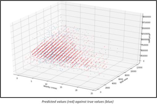
I did this in python with the sklearn library, which makes machine learning as simple as a few lines of code. Firstly, I had to split the data into training and testing sets, and decided on a split of 80% to 20%. Then I fitted the model using my test data. I was left with a set of coefficients : -8134.250231(crime) and 61.82510587(area), and an intercept of 422744.8249407327. I plotted the predicted values against the true values for my test set (~5000 entries) and obtained the following plot :
An astute observer would be able to see that the predicted values from a plane of sorts with the values given, and this is due to the simple fact that the predicted values are a simple 3D function, with two variables, and 3 coefficients that were calculated earlier. In fact, if one were to feed these 2 coefficients, the intercept as well as a range of x (nearby crimes) and y (total area) values in the limits defined by the graph itself (0–25 and 0–12000 respectively), then I should be able to produce a planar representation of the function :
This anonymous grey plane is a visual representation of my model, it is the best fit that could be found to predict sale prices while minimizing error. The equation to create this plot can be given in the following form :
There are a number of ways to evaluate the predictive ability of a model. For the purposes of this report, I will be using R2, or the coefficient of determination. It is the proportion of variance in the dependent variable that can be predicted from the independent variables. In the context of my problem, R2tells us what proportion of the variance of the sale price can be predicted by the nearby crimes and total area. For my purposes, I can simplify it as a measure of how close the predicted and true values of sale price are. The best possible R2 is 1.0, implying a perfect fit to every single data point. An R2score of 0 is equivalent to just having a mean line through your data. A negative R2score implies the fit is worse than a mean line through your data. I used the .score() function of sklearn to find the R2score of my model and got the following value : 0.08649959376111038.
A score of roughly 0.08 is not very good, in fact, it’s only marginally better than just a mean line through my data. These results, while disappointing, can be explained by the fact that there are a plethora of variables that affect price outside of the total area of the property and nearby crime rates. Things such as build date, neighborhood, amenities, material, floors, and many more all influence buyers decisions. Additionally, I am still not sure if I was able to effectively filter out the properties that were sold for nominal fees with my lower price floor of $15,000. My results with the Pearson correlation coefficient confirmed this, when I saw that total area and nearby crime were correlated, but only just. The model that was created would be very inefficient as an actual product, and more than likely not give very accurate predictions.
In the future, if I were to improve on this model, I would definitely start with a better dataset, the one I used had a relatively large proportion of fields in rows empty. I would also use a lot more variables in analysis, in order to best fit the data. However, I am pleased with the size of the dataset for the scope of my analysis.
The core problem of this project was to predict property prices using the crime rate in 12 months, and total area square feet. I used public domain data from Kaggle as input, wrangled and cleaned the data to make it suitable for input into my model. I used a multiple linear regression model, and arrived at a set of coefficients and intercepts. My model did not perform particularly well, however the results demonstrated that property prices are reliant on a vast number of variables, and trying to predict prices without accounting for all these variables will evidently not produce very good results.
This project was completed as part of the Coursera IBM Data Science Professional Certificate