Ensemble learning is a technique that combines predictions from multiple machine learning algorithms that uses bagging to make a more accurate prediction than a single model by reducing overfitting.
Overfitting is the process of fitting your model to training data so tightly that when you introduce new unseen data, the model does not perform very well. This is because overfit models tend to mistake noise and outliers in data for meaningful patterns.
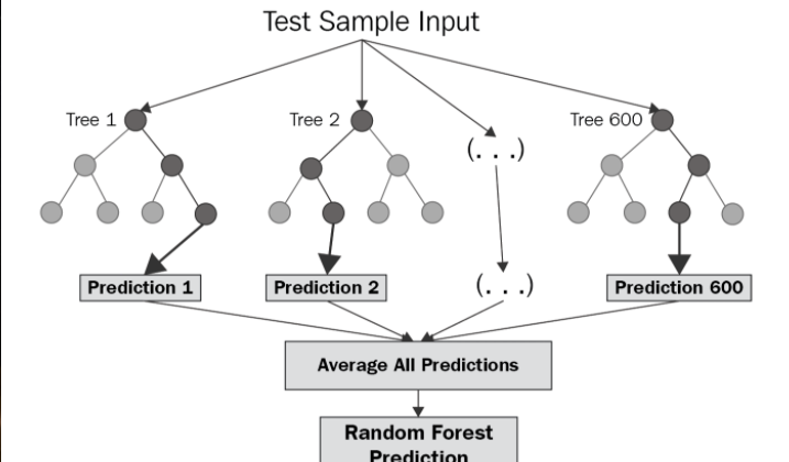
The diagram below shows the structure of an example ensemble model, in this case a Random Forest model. Notice how the final prediction is made up by averaging the results of multiple parallel decision trees.
This parallelism means ensemble models are more robust to overfitting than singular models. This is due to the fact each sub-model uses a sub-sample of the available training data, meaning models are less likely to converge on the same set of features.
You can either build all the sub-models at the same time, as is the case with Random Forest models, or you can try and improve performance further by building them additively (one after the other), actively trying to reduce the error with each new sub-model you build (known as differentiable loss function optimisation, or gradient descent).
The dataset for this exercise contained both categorical and numerical features (which is something that should be considered when assessing what type of ML model to use for an exercise). Tree-based models (such as AdaBoost, Random Forest or XGBoost) are well suited to mixed datasets since they branch on discriminative features. In my case I used an XGBoost model due to its speed on Python, gradient boosting optimisation and its regularization support. The last part especially is one of the reasons why XGBoost has such better performance than other similar libraries.
The loss function in this case was Root Mean Squared Logarithmic Error (RMSLE) rather than the commonly used Root Mean Square Error (RMSE). The reason for this is because RMSLE takes the logarithm of both predicted and actual sides. It does not penalise large differences if both predicted and actual values are also large, meaning the model produced will be more robust to predicting values for expensive properties in addition to normal ones.
After several iterations, I found the model predictions were nearly as accurate as those produced by our Property team, in a much shorter time!
Additionally, breaking down the patterns of the final models using SHAP values allowed us to understand patterns of rental values in much more detail, turning anecdotal suggestions into statistical evidence.
Our Engineering team moved this model into our production system, and the impact was instant! Our platform was now directing the Property team from thousands of potential candidates to the handful worth spending time on, meaning the team can fly through areas in search of the best investment cases.