Using the pix2pix architecture
Becker, Dan. (2017). Cityscapes Image Pairs Semantic Segmentation for Improving Automated Driving, Version 1. Retrieved December 3 2021 from https://www.kaggle.com/dansbecker/cityscapes-image-pairsSemantic Segmentation is one of the key concepts within computer vision. Semantic segmentation allows computers by color-coding objects in an image by type.
How are GANs suited to perform semantic segmentation?
GANs are built upon the concept of replicating and generating original content, based on real-world content. This makes them suitable for the task of semantic segmentation on street-view images. The segmentation of the different parts allow the agent that is navigating the environment to act suitably.
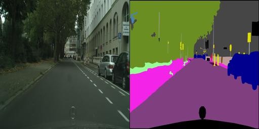
I accessed the data from a kaggle dataset, where the streetview, and the segmented images are paired together. This means that in order to construct the dataset, each image must be split in two, to split the semantic and streetview images of each instance.
from PIL import Image
from IPython.display import clear_output
import numpy as np
semantic = []
real = []
semantic_imgs = []
real_imgs = []
counter = 0
for img in img_paths:
if 'jpg' in img:
im = Image.open(img)
left = 0
top = 0
right = 256
bottom = 256
real_img = im.crop((left, top, right, bottom))
real_imgs.append(real_img)
real.append(np.array(real_img.getdata()).reshape(256,256,3))
left = 256
top = 0
right = 512
bottom = 256
semantic_img = im.crop((left, top, right, bottom))
semantic_imgs.append(semantic_img)
semantic.append(np.array(semantic_img.getdata()).reshape(256,256,3))
counter += 1
print(counter)
if counter % 10 == 0:
clear_output()
else:
print(img)
This script crops each image into two, and records the pixel value and the original image. The original image is also recorded, so that no further operation is needed to display it later.
import numpy as np
semantic = np.array(semantic)
real = np.array(real)X = real
y = semantic
After converting both of the lists into numpy array, one can directly define the X and y values. In fact, depending on your goal, you can switch the X and y values to control the model’s output. In this case, I want to convert the real images into semantic images. However I will try to train the GAN to convert semantic data into real data later.
from numpy import expand_dims
from numpy import zeros
from numpy import ones
from numpy import vstack
from numpy.random import randn
from numpy.random import randint
from keras.utils import plot_model
from keras.models import Model
from keras.layers import Input
from keras.layers import Dense
from keras.layers import Flatten
from keras.layers.convolutional import Conv2D,Conv2DTranspose
from keras.layers.pooling import MaxPooling2D
from keras.layers.merge import concatenate
from keras.initializers import RandomNormal
from keras.layers import LeakyReLU
from keras.layers import BatchNormalization
from keras.layers import Activation,Reshape
from keras.optimizers import Adam
from keras.models import Sequential
from keras.layers import Dropout
from IPython.display import clear_output
from keras.layers import Concatenate
As I am using the keras framework to construct the generator and the discriminator, I need to import all the necessary layer types to construct the model. This includes the main convolutional and convolutional transposition layers, as well as the batch normalization and leaky relu layers. The concatenate layer is used to construct the U-net architecture, as it can link certain layers together.
def define_discriminator(image_shape=(256,256,3)):
init = RandomNormal(stddev=0.02)
in_src_image = Input(shape=image_shape)
in_target_image = Input(shape=image_shape)
merged = Concatenate()([in_src_image, in_target_image])
d = Conv2D(64, (4,4), strides=(2,2), padding='same', kernel_initializer=init)(merged)
d = LeakyReLU(alpha=0.2)(d)
d = Conv2D(128, (4,4), strides=(2,2), padding='same', kernel_initializer=init)(d)
d = BatchNormalization()(d)
d = LeakyReLU(alpha=0.2)(d)
d = Conv2D(256, (4,4), strides=(2,2), padding='same', kernel_initializer=init)(d)
d = BatchNormalization()(d)
d = LeakyReLU(alpha=0.2)(d)
d = Conv2D(512, (4,4), strides=(2,2), padding='same', kernel_initializer=init)(d)
d = BatchNormalization()(d)
d = LeakyReLU(alpha=0.2)(d)
d = Conv2D(512, (4,4), padding='same', kernel_initializer=init)(d)
d = BatchNormalization()(d)
d = LeakyReLU(alpha=0.2)(d)
d = Conv2D(1, (4,4), padding='same', kernel_initializer=init)(d)
patch_out = Activation('sigmoid')(d)
model = Model([in_src_image, in_target_image], patch_out)
opt = Adam(lr=0.0002, beta_1=0.5)
model.compile(loss='binary_crossentropy', optimizer=opt, loss_weights=[0.5])
return model
This discriminator is a keras implementation of the model that the pix2pix GAN paper used. The use of leaky relu instead of normal relu is so that negative values are still taken into account. This increases the rate of convergence.
The discriminator performs binary classification, so sigmoid in the last layer and binary cross entropy as the loss function is used.
def define_encoder_block(layer_in, n_filters, batchnorm=True):
init = RandomNormal(stddev=0.02)
g = Conv2D(n_filters, (4,4), strides=(2,2), padding='same', kernel_initializer=init)(layer_in)
if batchnorm:
g = BatchNormalization()(g, training=True)
g = LeakyReLU(alpha=0.2)(g)
return gdef decoder_block(layer_in, skip_in, n_filters, dropout=True):
init = RandomNormal(stddev=0.02)
g = Conv2DTranspose(n_filters, (4,4), strides=(2,2), padding='same', kernel_initializer=init)(layer_in)
g = BatchNormalization()(g, training=True)
if dropout:
g = Dropout(0.5)(g, training=True)
g = Concatenate()([g, skip_in])
g = Activation('relu')(g)
return g
The generator consists of encoding the initial data multiple times, until you get a feature map of the original image. This feature image is then decoded, until you get a full resolution image. This means that most of the layers in the generator are just encoder and decoder blocks. After carefully engineering the encoder decoder blocks, there is not much more to do in order to construct the generator.
def define_generator(image_shape=(256,256,3)):
init = RandomNormal(stddev=0.02)
in_image = Input(shape=image_shape)
e1 = define_encoder_block(in_image, 64, batchnorm=False)
e2 = define_encoder_block(e1, 128)
e3 = define_encoder_block(e2, 256)
e4 = define_encoder_block(e3, 512)
e5 = define_encoder_block(e4, 512)
e6 = define_encoder_block(e5, 512)
e7 = define_encoder_block(e6, 512)
b = Conv2D(512, (4,4), strides=(2,2), padding='same', kernel_initializer=init)(e7)
b = Activation('relu')(b)
d1 = decoder_block(b, e7, 512)
d2 = decoder_block(d1, e6, 512)
d3 = decoder_block(d2, e5, 512)
d4 = decoder_block(d3, e4, 512, dropout=False)
d5 = decoder_block(d4, e3, 256, dropout=False)
d6 = decoder_block(d5, e2, 128, dropout=False)
d7 = decoder_block(d6, e1, 64, dropout=False)
g = Conv2DTranspose(3, (4,4), strides=(2,2), padding='same', kernel_initializer=init)(d7)
out_image = Activation('tanh')(g)
model = Model(in_image, out_image)
return model
Using multiple encoder and decoders, we get this generator. The use of the hyperbolic tangent is used to normalize the data, from the range of (0,255) to (-1,1). We must remember to encode the data to be in the range(-1,1), so the generator output and the y-values can be correctly evaluated.
def define_gan(g_model, d_model, image_shape):
d_model.trainable = False
in_src = Input(shape=image_shape)
gen_out = g_model(in_src)
dis_out = d_model([in_src, gen_out])
model = Model(in_src, [dis_out, gen_out])
opt = Adam(lr=0.0002, beta_1=0.5)
model.compile(loss=['binary_crossentropy', 'mse'], optimizer=opt)
return model
Connecting the two models together gives the full GAN. The output of the generator is directly fed into the discriminator.
def generate_real_samples(dataset, n_samples, patch_shape):
trainA, trainB = dataset
ix = randint(0, trainA.shape[0], n_samples)
X1, X2 = trainA[ix], trainB[ix]
y = ones((n_samples, patch_shape, patch_shape, 1))
X1 = (X1 - 127.5) / 127.5
X2 = (X2 - 127.5) / 127.5
return [X1, X2], ydef generate_fake_samples(g_model, samples, patch_shape):
X = g_model.predict(samples)
y = zeros((len(X), patch_shape, patch_shape, 1))
return X, y
For the discriminator to work, it must be fed both real samples and computer-generated samples. However, the process is not that simple, the values need to be normalized. Since the range of pixel values fall between 0 and 255, by using the equation X1 = (X1–127.5) / 127.5, all values will be normalized in the range (-1,1).
def train(d_model, g_model, gan_model, dataset, n_epochs=100, n_batch=10):
n_patch = d_model.output_shape[1]
trainA, trainB = dataset
bat_per_epo = int(len(trainA) / n_batch)
n_steps = bat_per_epo * n_epochs
for i in range(n_steps):
[X_realA, X_realB], y_real = generate_real_samples(dataset, n_batch, n_patch)
X_fakeB, y_fake = generate_fake_samples(g_model, X_realA, n_patch)
d_loss1 = d_model.train_on_batch([X_realA, X_realB], y_real)
d_loss2 = d_model.train_on_batch([X_realA, X_fakeB], y_fake)
g_loss, _, _ = gan_model.train_on_batch(X_realA, [y_real, X_realB])
print('>%d, d1[%.3f] d2[%.3f] g[%.3f]' % (i+1, d_loss1, d_loss2, g_loss))
if (i+1) % 100 == 0:
clear_output()
This function trains the GAN. The key thing to note here is the batch size. The paper suggested using minibatches (n_batch = 1) but after some testing, I found that a batch size of 10 would cause better results.
image_shape = (256,256,3)
d_model = define_discriminator()
g_model = define_generator()
gan_model = define_gan(g_model, d_model, image_shape)train(d_model, g_model, gan_model, [X,y])
This script defines the image shape and calls upon the functions to construct different parts of the GAN. It then calls upon the training function to train the model.
Real to Semantic:
Although the image that the computer generates is blurry, it correctly color-codes everything in the image. Keep in mind that the computer does not get to see the actual semantic representation of the real image! I think that the image is blurry, because the real 256 by 256 image is not very complex, as well as having many colors that could throw off the machine. The image on the right(computer generated) can be segmented into squares. If you count these squares, it would match up with the number of filters of the convolutional layers!