Machine learning model performance often improves with dataset size for predictive modeling.
This depends on the specific datasets and on the choice of model, although it often means that using more data can result in better performance and that discoveries made using smaller datasets to estimate model performance often scale to using larger datasets.
The problem is the relationship is unknown for a given dataset and model, and may not exist for some datasets and models. Additionally, if such a relationship does exist, there may be a point or points of diminishing returns where adding more data may not improve model performance or where datasets are too small to effectively capture the capability of a model at a larger scale.
These issues can be addressed by performing a sensitivity analysis to quantify the relationship between dataset size and model performance. Once calculated, we can interpret the results of the analysis and make decisions about how much data is enough, and how small a dataset may be to effectively estimate performance on larger datasets.
In this tutorial, you will discover how to perform a sensitivity analysis of dataset size vs. model performance.
After completing this tutorial, you will know:
- Selecting a dataset size for machine learning is a challenging open problem.
- Sensitivity analysis provides an approach to quantifying the relationship between model performance and dataset size for a given model and prediction problem.
- How to perform a sensitivity analysis of dataset size and interpret the results.
Let’s get started.

Sensitivity Analysis of Dataset Size vs. Model Performance
Photo by Graeme Churchard, some rights reserved.
Tutorial Overview
This tutorial is divided into three parts; they are:
- Dataset Size Sensitivity Analysis
- Synthetic Prediction Task and Baseline Model
- Sensitivity Analysis of Dataset Size
Dataset Size Sensitivity Analysis
The amount of training data required for a machine learning predictive model is an open question.
It depends on your choice of model, on the way you prepare the data, and on the specifics of the data itself.
For more on the challenge of selecting a training dataset size, see the tutorial:
One way to approach this problem is to perform a sensitivity analysis and discover how the performance of your model on your dataset varies with more or less data.
This might involve evaluating the same model with different sized datasets and looking for a relationship between dataset size and performance or a point of diminishing returns.
Typically, there is a strong relationship between training dataset size and model performance, especially for nonlinear models. The relationship often involves an improvement in performance to a point and a general reduction in the expected variance of the model as the dataset size is increased.
Knowing this relationship for your model and dataset can be helpful for a number of reasons, such as:
- Evaluate more models.
- Find a better model.
- Decide to gather more data.
You can evaluate a large number of models and model configurations quickly on a smaller sample of the dataset with confidence that the performance will likely generalize in a specific way to a larger training dataset.
This may allow evaluating many more models and configurations than you may otherwise be able to given the time available, and in turn, perhaps discover a better overall performing model.
You may also be able to generalize and estimate the expected performance of model performance to much larger datasets and estimate whether it is worth the effort or expense of gathering more training data.
Now that we are familiar with the idea of performing a sensitivity analysis of model performance to dataset size, let’s look at a worked example.
Synthetic Prediction Task and Baseline Model
Before we dive into a sensitivity analysis, let’s select a dataset and baseline model for the investigation.
We will use a synthetic binary (two-class) classification dataset in this tutorial. This is ideal as it allows us to scale the number of generated samples for the same problem as needed.
The make_classification() scikit-learn function can be used to create a synthetic classification dataset. In this case, we will use 20 input features (columns) and generate 1,000 samples (rows). The seed for the pseudo-random number generator is fixed to ensure the same base “problem” is used each time samples are generated.
The example below generates the synthetic classification dataset and summarizes the shape of the generated data.
|
# test classification dataset from sklearn.datasets import make_classification # define dataset X, y = make_classification(n_samples=1000, n_features=20, n_informative=15, n_redundant=5, random_state=1) # summarize the dataset print(X.shape, y.shape) |
Running the example generates the data and reports the size of the input and output components, confirming the expected shape.
Next, we can evaluate a predictive model on this dataset.
We will use a decision tree (DecisionTreeClassifier) as the predictive model. It was chosen because it is a nonlinear algorithm and has a high variance, which means that we would expect performance to improve with increases in the size of the training dataset.
We will use a best practice of repeated stratified k-fold cross-validation to evaluate the model on the dataset, with 3 repeats and 10 folds.
The complete example of evaluating the decision tree model on the synthetic classification dataset is listed below.
|
# evaluate a decision tree model on the synthetic classification dataset from sklearn.datasets import make_classification from sklearn.model_selection import cross_val_score from sklearn.model_selection import RepeatedStratifiedKFold from sklearn.tree import DecisionTreeClassifier # load dataset X, y = make_classification(n_samples=1000, n_features=20, n_informative=15, n_redundant=5, random_state=1) # define model evaluation procedure cv = RepeatedStratifiedKFold(n_splits=10, n_repeats=3, random_state=1) # define model model = DecisionTreeClassifier() # evaluate model scores = cross_val_score(model, X, y, scoring=‘accuracy’, cv=cv, n_jobs=–1) # report performance print(‘Mean Accuracy: %.3f (%.3f)’ % (scores.mean(), scores.std())) |
Running the example creates the dataset then estimates the performance of the model on the problem using the chosen test harness.
Note: Your results may vary given the stochastic nature of the algorithm or evaluation procedure, or differences in numerical precision. Consider running the example a few times and compare the average outcome.
In this case, we can see that the mean classification accuracy is about 82.7%.
|
Mean Accuracy: 0.827 (0.042) |
Next, let’s look at how we might perform a sensitivity analysis of dataset size on model performance.
Sensitivity Analysis of Dataset Size
The previous section showed how to evaluate a chosen model on the available dataset.
It raises questions, such as:
Will the model perform better on more data?
More generally, we may have sophisticated questions such as:
Does the estimated performance hold on smaller or larger samples from the problem domain?
These are hard questions to answer, but we can approach them by using a sensitivity analysis. Specifically, we can use a sensitivity analysis to learn:
How sensitive is model performance to dataset size?
Or more generally:
What is the relationship of dataset size to model performance?
There are many ways to perform a sensitivity analysis, but perhaps the simplest approach is to define a test harness to evaluate model performance and then evaluate the same model on the same problem with differently sized datasets.
This will allow the train and test portions of the dataset to increase with the size of the overall dataset.
To make the code easier to read, we will split it up into functions.
First, we can define a function that will prepare (or load) the dataset of a given size. The number of rows in the dataset is specified by an argument to the function.
If you are using this code as a template, this function can be changed to load your dataset from file and select a random sample of a given size.
|
# load dataset def load_dataset(n_samples): # define the dataset X, y = make_classification(n_samples=int(n_samples), n_features=20, n_informative=15, n_redundant=5, random_state=1) return X, y |
Next, we need a function to evaluate a model on a loaded dataset.
We will define a function that takes a dataset and returns a summary of the performance of the model evaluated using the test harness on the dataset.
This function is listed below, taking the input and output elements of a dataset and returning the mean and standard deviation of the decision tree model on the dataset.
|
# evaluate a model def evaluate_model(X, y): # define model evaluation procedure cv = RepeatedStratifiedKFold(n_splits=10, n_repeats=3, random_state=1) # define model model = DecisionTreeClassifier() # evaluate model scores = cross_val_score(model, X, y, scoring=‘accuracy’, cv=cv, n_jobs=–1) # return summary stats return [scores.mean(), scores.std()] |
Next, we can define a range of different dataset sizes to evaluate.
The sizes should be chosen proportional to the amount of data you have available and the amount of running time you are willing to expend.
In this case, we will keep the sizes modest to limit running time, from 50 to one million rows on a rough log10 scale.
|
... # define number of samples to consider sizes = [50, 100, 500, 1000, 5000, 10000, 50000, 100000, 500000, 1000000] |
Next, we can enumerate each dataset size, create the dataset, evaluate a model on the dataset, and store the results for later analysis.
|
... # evaluate each number of samples means, stds = list(), list() for n_samples in sizes: # get a dataset X, y = load_dataset(n_samples) # evaluate a model on this dataset size mean, std = evaluate_model(X, y) # store means.append(mean) stds.append(std) |
Next, we can summarize the relationship between the dataset size and model performance.
In this case, we will simply plot the result with error bars so we can spot any trends visually.
We will use the standard deviation as a measure of uncertainty on the estimated model performance. This can be achieved by multiplying the value by 2 to cover approximately 95% of the expected performance if the performance follows a normal distribution.
This can be shown on the plot as an error bar around the mean expected performance for a dataset size.
|
... # define error bar as 2 standard deviations from the mean or 95% err = [min(1, s * 2) for s in stds] # plot dataset size vs mean performance with error bars pyplot.errorbar(sizes, means, yerr=err, fmt=‘-o’) |
To make the plot more readable, we can change the scale of the x-axis to log, given that our dataset sizes are on a rough log10 scale.
|
... # change the scale of the x-axis to log ax = pyplot.gca() ax.set_xscale(“log”, nonpositive=‘clip’) # show the plot pyplot.show() |
And that’s it.
We would generally expect mean model performance to increase with dataset size. We would also expect the uncertainty in model performance to decrease with dataset size.
Tying this all together, the complete example of performing a sensitivity analysis of dataset size on model performance is listed below.
|
1 2 3 4 5 6 7 8 9 10 11 12 13 14 15 16 17 18 19 20 21 22 23 24 25 26 27 28 29 30 31 32 33 34 35 36 37 38 39 40 41 42 43 44 45 46 47 |
# sensitivity analysis of model performance to dataset size from sklearn.datasets import make_classification from sklearn.model_selection import cross_val_score from sklearn.model_selection import RepeatedStratifiedKFold from sklearn.tree import DecisionTreeClassifier from matplotlib import pyplot
# load dataset def load_dataset(n_samples): # define the dataset X, y = make_classification(n_samples=int(n_samples), n_features=20, n_informative=15, n_redundant=5, random_state=1) return X, y
# evaluate a model def evaluate_model(X, y): # define model evaluation procedure cv = RepeatedStratifiedKFold(n_splits=10, n_repeats=3, random_state=1) # define model model = DecisionTreeClassifier() # evaluate model scores = cross_val_score(model, X, y, scoring=‘accuracy’, cv=cv, n_jobs=–1) # return summary stats return [scores.mean(), scores.std()]
# define number of samples to consider sizes = [50, 100, 500, 1000, 5000, 10000, 50000, 100000, 500000, 1000000] # evaluate each number of samples means, stds = list(), list() for n_samples in sizes: # get a dataset X, y = load_dataset(n_samples) # evaluate a model on this dataset size mean, std = evaluate_model(X, y) # store means.append(mean) stds.append(std) # summarize performance print(‘>%d: %.3f (%.3f)’ % (n_samples, mean, std)) # define error bar as 2 standard deviations from the mean or 95% err = [min(1, s * 2) for s in stds] # plot dataset size vs mean performance with error bars pyplot.errorbar(sizes, means, yerr=err, fmt=‘-o’) # change the scale of the x-axis to log ax = pyplot.gca() ax.set_xscale(“log”, nonpositive=‘clip’) # show the plot pyplot.show() |
Running the example reports the status along the way of dataset size vs. estimated model performance.
Note: Your results may vary given the stochastic nature of the algorithm or evaluation procedure, or differences in numerical precision. Consider running the example a few times and compare the average outcome.
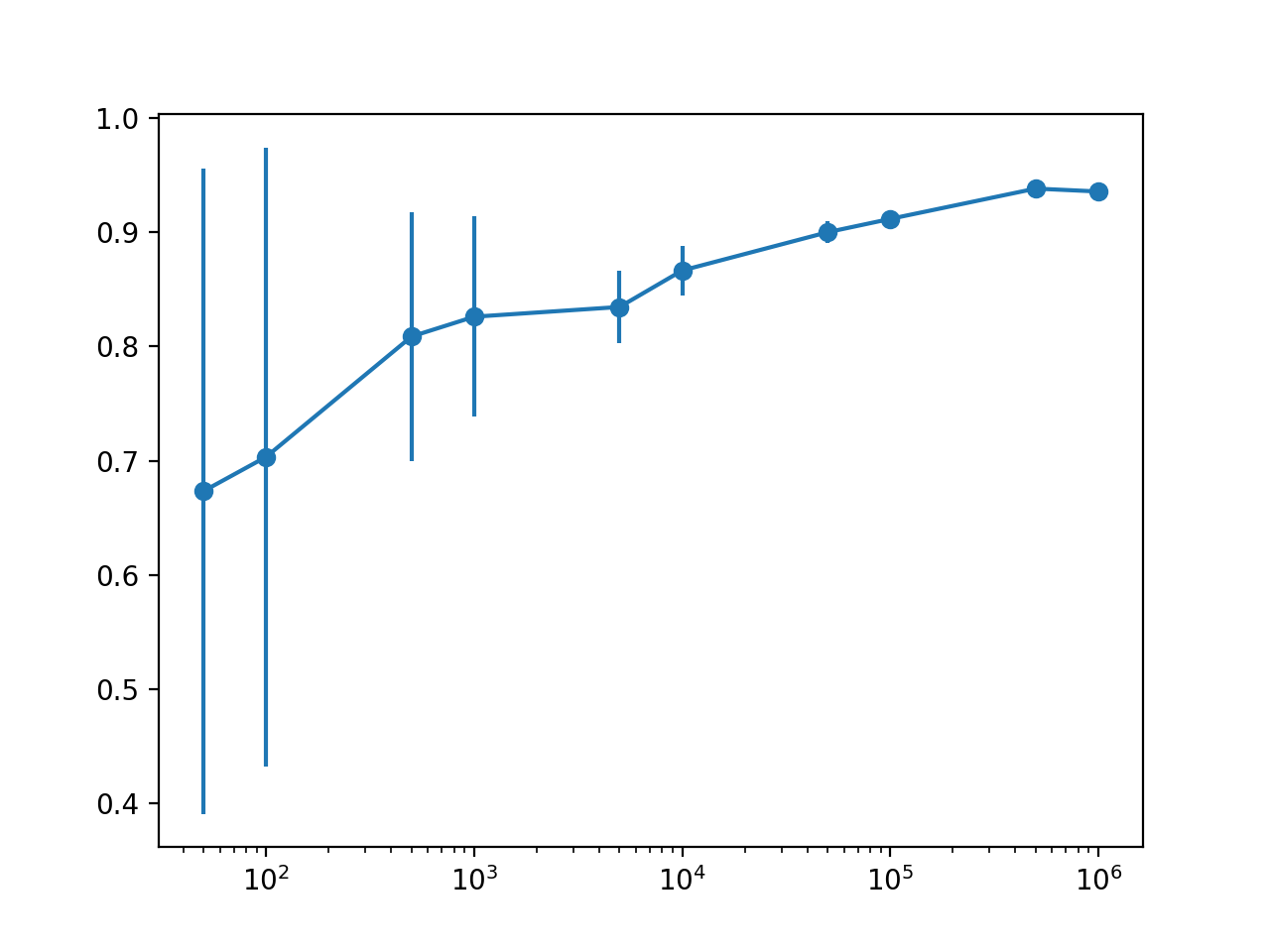
In this case, we can see the expected trend of increasing mean model performance with dataset size and decreasing model variance measured using the standard deviation of classification accuracy.
We can see that there is perhaps a point of diminishing returns in estimating model performance at perhaps 10,000 or 50,000 rows.
Specifically, we do see an improvement in performance with more rows, but we can probably capture this relationship with little variance with 10K or 50K rows of data.
We can also see a drop-off in estimated performance with 1,000,000 rows of data, suggesting that we are probably maxing out the capability of the model above 100,000 rows and are instead measuring statistical noise in the estimate.
This might mean an upper bound on expected performance and likely that more data beyond this point will not improve the specific model and configuration on the chosen test harness.
|
>50: 0.673 (0.141) >100: 0.703 (0.135) >500: 0.809 (0.055) >1000: 0.826 (0.044) >5000: 0.835 (0.016) >10000: 0.866 (0.011) >50000: 0.900 (0.005) >100000: 0.912 (0.003) >500000: 0.938 (0.001) >1000000: 0.936 (0.001) |
The plot makes the relationship between dataset size and estimated model performance much clearer.
The relationship is nearly linear with a log dataset size. The change in the uncertainty shown as the error bar also dramatically decreases on the plot from very large values with 50 or 100 samples, to modest values with 5,000 and 10,000 samples and practically gone beyond these sizes.
Given the modest spread with 5,000 and 10,000 samples and the practically log-linear relationship, we could probably get away with using 5K or 10K rows to approximate model performance.

Line Plot With Error Bars of Dataset Size vs. Model Performance
We could use these findings as the basis for testing additional model configurations and even different model types.
The danger is that different models may perform very differently with more or less data and it may be wise to repeat the sensitivity analysis with a different chosen model to confirm the relationship holds. Alternately, it may be interesting to repeat the analysis with a suite of different model types.
Further Reading
This section provides more resources on the topic if you are looking to go deeper.
Tutorials
APIs
Articles
Summary
In this tutorial, you discovered how to perform a sensitivity analysis of dataset size vs. model performance.
Specifically, you learned:
- Selecting a dataset size for machine learning is a challenging open problem.
- Sensitivity analysis provides an approach to quantifying the relationship between model performance and dataset size for a given model and prediction problem.
- How to perform a sensitivity analysis of dataset size and interpret the results.
Do you have any questions?
Ask your questions in the comments below and I will do my best to answer.

