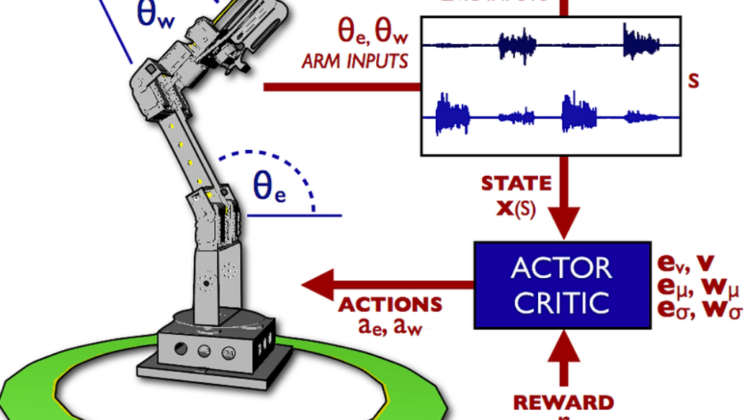
Solving Continuous Control using Deep Reinforcement Learning (Policy-Based Methods)

Training Loop

For episode e ⟵1 to M:

Initialize a random process N for action exploration
Receive initial observation state, s1

for i_episode in range(1, n_episodes + 1):   env_info = env.reset(train_mode=True)[brain_name]
states = env_info.vector_observations          
score = np.zeros(n_agents)

Here we are able to sample our initial environment state as well as set up a list to store our training scores.

For step t ⟵ 1 to T:

for t in range(max_t):            
actions = agent.act(states)                                   
env_info = env.step(actions)[brain_name]                    
next_states = env_info.vector_observations    
rewards = env_info.rewards
dones = env_info.local_done
agent.step(states, actions, rewards, next_states, dones)                                   
score += env_info.rewards                    
states = next_states
if np.any(dones): # Check if there are any done agents                          
break

Select action A= µ(st|θ-µ) + Noise according to the current policy and exploration noise

Here we use the local Actor model to sample an action space with a bit of added noise exploration. For the noise added to the actions, DDPGs often use the Ornstein–Uhlenbeck process to generate temporally correlated exploration for exploration efficiency in physical control problems.

Execute action at and observe reward r(t) and observe new state s (t+1), where t is the current timestep

    env_info = env.step(actions)[brain_name]                    
next_states = env_info.vector_observations    
rewards = env_info.rewards
dones = env_info.local_done

Store transition s(t), a(t), r(t), s(t+1)] in Replay Buffer, R

agent.step(states, actions, rewards, next_states, dones)

The remaining parts are the algorithm are mathematical learning steps to update the policy (weights of the local and target networks).

Learning Steps of DDPG Algorithm

The agent takes a step and immediately samples randomly from the replay buffer to learn a bit more about the environment it is currently in. We can split the update into two parts: Actor and Critic update. (Note: Actor loss is -ve due to the fact we are trying to maximize the return values passed by the Critic.)

DDPG only updates the local networks (the networks that interact with the environment) and performs soft updates on the target networks. As you can see below, soft updates only factor in a small amount of the local networks weights (defined by Tau).

Yeah, so that’s it! The model is able to learn over time and develop the ability to follow a goal location in a continuously controlled state. The full repository can be viewed here.

Plot of Results

Training Parameters:

Max Episodes: 1500
Max Time Steps: 3000
Buffer Size: 10000
Batch Size: 128
Gamma: 0.99
Tau: 1e-3
Actor Learning Rate = 1e-3
Critic Learning Rate = 1e-3
Weight Decay: 0.0

Training Progression

This concludes the exploration of continuous control using reinforcement learning algorithms. Continuous control is just one of several applications that Actor-Critic methods strive in tackling. Please check out my previous post, where I tackle Naviagation using Deep RL.

Footer