You have probably heard of the term “Machine Learning” by now. In case you haven’t, Machine Learning (ML) concerns the study of computer algorithms that learn to perform tasks with experience, rather than explicit programming. Advances in computational power over the past decade have led to a resurgence of the field and it seems that it is now set to become one of the most transformative technologies of this decade.
Much of the hype around ML today revolves around what is called “Neural Networks”. While Neural Networks are certainly an important subset of ML algorithms, they are often outperformed by classical ML algorithms. One such algorithm is the Support Vector Machine (SVM) which tends to outperform Neural Networks in most classification problems. In this article, we’ll be delving into the basics of SVMs.
SVM is a supervised ML algorithm that has found wide usage due to its simplicity, effectiveness, and inexpensive computational footprint. Although it can be used for both classification and regression tasks, it tends to be used more for the former. In the real world, it is employed in applications for Face Detection, Text Categorization, Handwriting Recognition and more. The primary objective with SVMs is to:
Find the optimal hyperplane that can classify the data in our feature space.
Let’s break it down!
Hyperplane
A hyperplane is, in essence, a decision boundary for our data. The utility of a decision boundary is evident from its name. It allows us to make decisions on data points based on the side of the boundary that they lie on. For example, if our decision boundary is: number of wheels = 3, data points that lie to the left of the decision boundary likely come from bikes, and those on the right likely come from cars.
For complex data sets with over 3 dimensions, it is difficult to visualize the separating hyperplane. Nevertheless, the intuition carries!
Feature Space
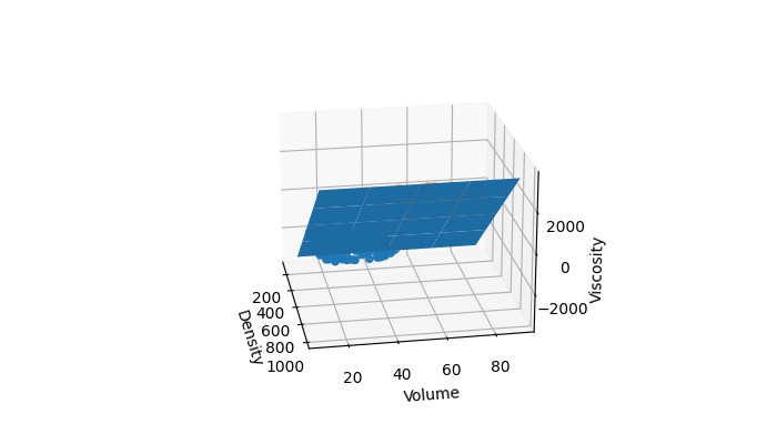
Moving on, the feature space denotes the space where all our data points come from. For example, say our data contains the volume, density, and viscosity for two liquids. The feature space for our data would be 3 dimensional; the first dimension being “volume”, the second “density”, and the third “viscosity”. All positive values for the three dimensions would comprise our feature space (space where all our observations come from). See the illustration below which shows where our data points exist in the feature space.
The Process
There are usually several hyperplanes that can be used to classify data. The SVM finds the optimal hyperplane by maximizing the total distance between the hyperplane and the data points surrounding it, which are called support vectors. This allows us to find a hyperplane that is more likely to be robust to unfamiliar data. For the data shown earlier, here is the hyperplane that was found by a linear SVM.
While most of the mathematical details that go into creating an SVM are abstracted away from users by ML libraries, it is important to note that using SVMs in real-world projects will require some knowledge of the underlying mathematics and encounters with complex datasets that have more than 2 or 3 dimensions. Regardless, the ideas mentioned in the article should be enough to get you started!
If you would like to get your hands dirty with the SVM implementation and visualizations in this article, you can find them here. If you have any feedback or ideas you’d like me to cover, you can send them to me here. I’ve also compiled a list of other useful resources that can help you dive further into SVMs so you can use them for your own projects:
Thanks for reading till the end! Happy Learning!