BERT is a prize addition to the practitioner’s toolbox
Natural language processing tasks traditionally requiring labeled data could be solved entirely or in part, subject to a few constraints, without the need for labeled data by leveraging the self-supervised learning of a BERT model, provided those tasks lend themselves to be viewed entirely or in part, as a similarity measure problem.
An example of a task that can be viewed entirely as a similarity measure problem, other than semantic search (which is inherently similarity measure), is a sequence tagging problem like NER. While certain kinds of sentence classification tasks could be viewed as a similarity measure problem, sentiment classification cannot leverage off similarity measure, given a BERT model clusters concepts disregarding their negative or positive sentiment and is unable to reliably separate them even given full sentence context. Harvesting a graph that is not based on similarity measure (e.g. dependency parser), is also out of scope (although it is possible to harvest a dependency graph with a transformation learned with supervision). However, a dependency parser used in concert with similarity measure (for detecting entity types a dependency parser edges link) could be used for relation extraction.
This post is a review of some of the tasks where self-supervised learning of BERT is leveraged to solve a task entirely or in part. These tasks are typically solved with labeled data by fine-tuning BERT — its predominant use for NLP task solving.
There are excellent detailed articles online on BERT and transformer models in general.
The focus in this section is on BERT’s inner workings that could be leveraged off to avoid labeled data in traditionally supervised NLP tasks.
A key step prior to pre-training a BERT model from scratch is the choice of a vocabulary that best represents the corpus to be used for training. This is typically around 30,000 terms composed of characters, full words and partial words (subwords) that can be stitched to compose full words. Any input to the model would be constructed using these ~30,000 terms (if the input contains a term that cannot be decomposed into these 30k terms, it would be represented as a special unknown token that is also part of this set. An example is say a Chinese character that is not present in the 30k set).
During training,
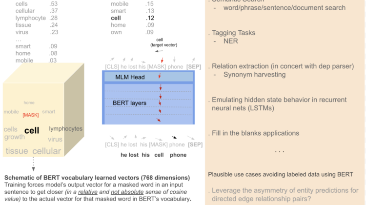
- the model learns a vector representation for all the terms in its vocabulary. This learning is facilitated by the decomposition of sentences in the input training corpus into terms in the vocabulary (tokenization) as each sentence is fed into the model. Prior to training, model starts with a random vector representation of each term in its vocabulary, which by virtue of the high dimension (e.g . 768) of those vectors makes them nearly orthogonal to each other (essentially a dense representation that behaves like a one-hot vector where each vocabulary term is represented uniquely and almost orthogonal to all other terms).
- the model learns a transformation composed of all the layers of a BERT model. This learned transformation (which is essentially learning weights that implement the transformation), is a function that takes in vectors representing each of the tokenized terms in an input sentence (the vectors mentioned in previous bullet) and produces transformed output vectors for each input vector. During training, roughly 15% of those input vectors are either replaced by a placeholder vector or by the vector for another word (picked randomly from the vocabulary) and the transformation is forced to produce an output vector (leveraging the context provided by other vectors in the input sentence) that can be scored, relative to the other vocabulary vectors, to predict the same original vector that was replaced. The cosine distance between the output vector and the original vector that was masked/replaced, is the key factor in determining the score. The angle between the top scoring output vector for a masked/replaced position and the actual vocabulary vector(the vector being predicted) can be, counterintuitively, closer to being orthogonal than collinear — i.e. as high as 80 degrees apart. Yet relative to other vocabulary vectors it still makes the output vector, the best prediction (figure 5).
- A key fact is both the vector representations of vocabulary terms and the model transformation weights are learned simultaneously. This at first glance may seem odd, given the learning of the transformation depends on the vocabulary vectors serving both as reference vectors on the output side and representing sentences on the input side, while those vocabulary vectors are themselves changing. This simultaneous learning approach works because very few tokens in a sentence are replaced by placeholder/random word vectors during training (~15%). So each vocabulary vector gets much more opportunity to converge to a stable representation by participating from the input end in the prediction of a replaced vector than itself being used as a reference vector on the output end for a transformed replaced vector to gravitate towards it. Once training is done, these vocabulary vectors serve as static landmark vectors to deduce the meaning of an output vector explained in detail below.
- Another interesting fact, even though the same target vector for a word is used to influence the learning of the contextually different meanings of a word, the word vectors in the vocabulary capturing the contextually different meanings are not necessarily mixed together in a cluster — a useful property that is leveraged off in the unsupervised applications described below. For instance, the cosine neighborhood for the word cell (in a model that was pre-trained from scratch with a custom vocabulary on a biomedical domain corpus) in the vocabulary vector space is largely biological terms(figure 4). Terms capturing the other meanings (cell phone, prison cell) are far away from the vector cell. This is in stark contrast to a model like word2vec where all the senses(meanings) of a word would be mixed in the top neighborhood. However, in some cases mixing of senses can be also observed in the underlying learned vocabulary like a word2vec model. For instance, the cosine neighborhood in the learned vocabulary vector space, for the term her is a mixture of two senses — pronouns and genes — his, she, hers, erbb, her2 (figure 2). This is a consequence of the fact that in an uncased model, HER — a gene, gets converted to her, increasing the ambiguity with the pronoun her. However, the transformation still separates these senses based on sentence context (this is assuming the sentence contexts for the two different meanings are different). In summary, for each term in the input sentence, the learned transformation finds a new vector for a masked/replaced term, relative to which the cosine neighborhood in the vocabulary vector space is composed of semantically similar terms, by leveraging the sentence context, regardless of the fact the semantically different meanings of the masked term is clustered or separated in the vocabulary vector space (although in most cases in a well trained model, vocabulary vector clusters tend to capture a single entity sense, to a certain level of granularity)
One can see the transformation in full action in a single sentence where all the different meanings of a cell emerge based on its position/context within the sentence. Attention — a key component of the transformation is central to accomplish this. By performing a weighted sum of specific terms in the sentence (where the weights are not static learned weights but dynamic weights created as function of the words in the sentence) for each occurrence of the cell, the different contextual meanings of the word cell are captured.
he went to prison cell with a cell phone to draw blood cell samples from inmates
A consequence of the training process described above, which makes BERT the Swiss army knife, is the vocabulary vectors largely form entity specific clusters as well as clusters capturing syntactic similarities. The nature of these clusters are influenced by both the corpus it is trained on as well as the hyper parameters of the training process such as the batch size, learning rate, number of training steps etc. These clusters can be labeled based (details of the clustering in additional notes below) on the application of interest — a one time process. Used in conjunction with the learned transformation they facilitate conversion of traditionally labeled data problems into unsupervised tasks.
Unsupervised NER, explained in detail in this article, simply leverages off the clustering properties of a trained BERT model’s vocabulary to label model’s prediction for terms in a sentence.
It should be possible to apply the same approach for unsupervised POS, at least for a few coarse-grained tag types that can be distinguished by the different clusters of BERT’s vocabulary. The singular and plural versions of tags would be indistinguishable since they would cluster into the same group. The transformation would not be able to separate them in this case, since the sentence contexts for the singular and plural versions are nearly the same.
One detail that is perhaps key to not miss when evaluating the vectors of pre-trained model is where to harvest the output vectors of the model from. The right place is from the masked MLM head (captured in a PyTorch dump as cls.predictions). This is because there is one more transformation in that head prior to predicting the output vector. This transformation is ignored for subsequent fine-tuning, as it should be, but is key for evaluating or directly using the pre-trained output vectors. The unsupervised tasks in this article utilize either directly or indirectly vector outputs from MLM head (for all tokens including [CLS]) as opposed to the topmost layer vectors.
One task where the model’s pre-trained output vector is typically directly used is the [CLS] vector. This vector learns a representation for the entire sentence by predicting the next sentence in the input (all inputs to the model during training are sentence pairs with a flag indicating if the two sentences are contiguous). Harvesting this vector to represent a sentence from the MLM head as opposed to the topmost layer makes a difference in the performance given the additional transformation in the MLM head mentioned above.
The [CLS] vector harvested from the MLM head after pre-training, particularly from a model with a high next sentence prediction accuracy can be used to represent a word, phrase, or sentence. This has some advantages
- it expands the model’s ability to create representations effectively for an infinite vocabulary (with the caveat of representing symbols not present in the base vocabulary as the special [UNK] token )
- Unlike other learned sentence representations that are typically opaque, this representation is interpretable to some degree — we can get a sense of what a [CLS] representation is capturing by examining the neighborhood terms of the vectors in BERT’ vocabulary (or the clusters of BERT’s vocabulary). The learned model bias weights come in handy to weight such a neighborhood as explained below.
As an aside, the [CLS] output appears to be prematurely harvested in few papers and publicly available implementations (references below) from the topmost layer as opposed to the MLM head when creating sentence representations. This may in part be the reason [CLS] vectors perform poorly in such evaluations (this claim needs to be confirmed by testing with a benchmark like STS).
Relation extraction
If we consider a relation to be a three-tuple of phrases (e1,relation,e2), potentially occurring in any permutation of the three tuples, the identification of entities e1 and e2 can be done using unsupervised NER described above. The identification of the relation can be done by choosing the terms characterizing a specific relation in the vocabulary space — a one time step. A dependency parser would be required to identify the three tuples in a sentence and to find the relation boundaries, particularly when the relation is present in prefix(relation e1 e2) or post fix form (e1 e2 relation). This approach is used to harvest synonyms as described in this post. Another plausible use case is not necessarily to extract a relation but to identify the type of relation in a sentence in order to classify the sentence.
Emulating hidden state behavior of an RNN
[CLS] vector could be used to emulate the hidden state of an RNN at every time step with BERT which is just a Transformer encoder — a functionality that typically requires both an encoder and decoder when using a Transformer (e.g. in translation) . This could be useful in applications with temporal input streams. This is illustrated with partial and complete versions of a couple of toy sentences below (figures 11a-11d) where the neighborhood for [CLS] vector largely reflects semantically related terms of important entities in the input. This however may only be a crude approximation, given the autoregressive training of an RNN based language model endows it with generative capacity, that an auto encoder model like BERT clearly lacks.
Fill in the blanks application (for entity guessing)
This is simply the direct use of the MLM head as illustrated in many examples above. While the model performs quite well in predicting the entity type for any masked position, the accuracy of the prediction from a factual correctness of the entity instance cannot be relied upon, regardless of the fact in many instances, the predictions may fall within the range of the correct instance. For instance, in the example above “aripiprazole is used to treat”, the neighbors reflect diseases that are largely mental disorders. This could be of potential value to harvest instance candidates that can then be used to identify exact instance by a downstream model.
Miscellaneous model properties that could be of value
Utilizing learned bias values in MLM head
The output score during prediction of a masked position, is the dot product of the output vector and the vocabulary vectors with the addition of a bias value specific to each vocabulary word — the bias value is learned during training. Terms like the, the symbol for comma, and are part of the output predictions in many locations in a sentence — their information content is low. This learned bias could be of value to weight the predicted terms for a position in a sentence — serving like a TF-IDF for vocabulary terms.
The output vector angles with the vocabulary vectors is the primary factor in determining the model prediction for a position, with the learned bias and the vocabulary vector magnitude playing the secondary role.
Asymmetry of relative importance between representation pairs
Affinity graph of output vectors for tokens in a sentence
Non-commutativity of entity pairs in specific sentence contexts
All applications above leverage off similarity measure on learned vectors. Specifically, similarity measure is applied on learned distributed representations, and learned transformation of those distributed representations — both this learning being self-supervised. While any understanding of language baked into those representations and transformations is limited to only what can be gleaned from token sequences, that limited understanding still proves to be useful for solving a variety of NLP tasks without supervision.