- Introduction
Momentum investing/trading strategy is a strategy in which an investor buys liquid securities (such as stocks) that are showing an upward trend in their prices and sells those that show downward trend in their prices. One of the main goals of momentum investing is to forecast the price trend of stocks in order to formulate a strategy to enter and exit from an investment in a timely manner.
In this work, we seek to develop short-term momentum trading strategies to invest in stocks. We investigate the most popular blue-chip stocks called the FANG (Facebook, Apple, Netflix and Google) stocks. The objective is to forecast the near-future prices (1-day, 3-day, 5-day and 7-day forecasts) of FANG stocks using Apache Spark Machine Learning libraries and historical daily-price data from 2008 to 2018 obtained from Nasdaq.com. The forecast will be used to formulate simple short-term trading strategies
2. Description of Software/Tools
Quandl package
We use data from Nasdaq.com. For this purpose, we use a package called quandl [1]. This package has been acquired by Nasdaq.com. This is a popular database for financial time-series data and provides Python and R APIs for downloading the data and for performing simple manipulations on the data [2]. We use the Python-time-series API for obtaining the data [3].
Installation:
We can install from the PyPI or github repository using
$pip install quandl
Using the package:
We simply import the quandl package using the import command in our Python client program.
import quandl
Authentication:
In order to access the data using the quandl APIs, we need to create an account in the quandl website [1], and generate an authentication key. We need to set the authentication key in the python client program as follows,
quandl.ApiConfig.api_key = “your API key”
Querying data:
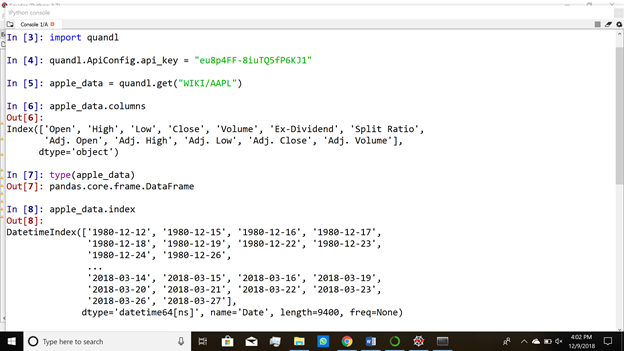
We query the data using the quandl python APIs. The queried data is obtained as a pandas dataframe. For example, we can obtain the time-series data of apple stock price as follows,
apple_data = quandl.get(“WIKI/AAPL”)
apple_data is a pandas dataframe and has “Date” column as its index (of datetime data type). We need to reset the index if we need use the “Date” column in our calculations (Figure 1a).
If we need to obtain data from a specified time frame (Figure 1b), we can make filtered time-series call [3],
apple_data_timeframe = quandl.get(“WIKI/AAPL”,start_date = ‘2014–09–01’, end_date = ‘2015–09–01’)
Also, if we need to make any transformations to the data while querying, we can append the call with the transformation type [3]. For example, if we need differenced data (i.e. yt — yt-1), the command is (Figure 1c),
apple_data_diff = quandl.get(“WIKI/AAPL”,transformation = ‘diff’)
Furthermore, we can change the frequency of the time-series data but appending the get call with frequency argument. For instance, we can obtain data with daily, weekly, monthly frequency etc. We can also download the data files as CSV files using an Excel add-in. Thus, the quandl package provides set of easy-to-use APIs for obtain financial time-series data from Nasdaq.com.
In addition to quandl package, we use PySpark in Anaconda (Spyder version 3.3.2, Jupyter version 5.6.0) and also use VMWare Workstation with CentOS 7.5 VM
3. Description of Data and Exploratory data analysis
We look at the stock prices of four stocks, Apple, Facebook, Netflix and Google and perform a brief exploratory data analysis. We perform simple tests to determine the stationarity of the time-series. We treat each stock price as a univariate time-series.
We first check for null values in the dataset. We first explore Facebook’s stock price data. We see that we have daily closing price data starting from 2012–05–18 till 2018–03–27 and there are no null values in the dataset.
Similarly, we check the datasets for Apple, Netflix and Google stock prices.
We have daily closing price data for Netflix stock starting from 2002–05–23 till 2018–03–27. There are no null values in the Netflix dataset. For Apple stock, we have daily closing price data ranging from 1980–12–12 till 2018–03–27 and there are no null values in the Apple dataset. Finally, for Google stock, we have daily closing price data ranging from 2004–08–19 till 2018–03–27. There are no null values in the Google dataset.
Checking for stationarity of time-series:
We perform augmented Dickey-Fuller’s test to find if the time-series data is stationary. We observe that all the four stocks price time-series are non-stationary.
We accept the null hypothesis, i.e. the time-series data is stationary if p-value > 0.05. Following are the summary of results:
Although the complete time series data is non-stationary, there could be parts of data that are stationary.
We make the time-series data approximately stationary by obtaining the first difference of the data. First difference is defined as follows,
If St is the stock price at time-step t, then first difference, Zt = St — St-1
This method of making the series stationary is an approximate one and would work only if the time-series is difference-stationary. However, stock price data are known to be highly non-stationary. They could exhibit trends, seasonality etc. We do not explore these aspects in this work.
After performing first differencing on the raw stock price data, we employ machine learning algorithms on the differenced data. This method is known to yield stable, reliable forecasts. To check if the differenced data is stationary, we again perform augmented Dickey-Fuller’s test on the differenced data. We see that differenced data is stationary. All the p-values are less 0.05 and ADF statistic values are highly negative and less than 1% critical value (see Figure 2h, 2i). This suggests that we should work with differenced data for time-series forecasting.
We compare the rolling mean of raw price data and differenced stock price data of Google stock. We see that upon differencing the 30-day rolling mean is somewhat constant for differenced data (implying that differenced data is stationary, and we have de-trended it).
However, there is not much difference in the standard deviation.
Similarly, for Apple stock, we see that upon differencing the data, we remove the trend in stock price and make it stationary. We see that 30-day rolling mean for differenced data is mostly constant (except in the end).
We see that variance of Apple stock price doesn’t change much upon differencing the data (as we saw before Google stock price).
Thus, we conclude that by differencing the time-series data we can make it stationary and hence avoid spurious regression. In the next part of the series, we will describe, in detail, the classes and utility functions we developed to perform time-series forecasting using Spark MLlib.
References:
[1] www.quandl.com