Continuing on the work of my previous post, I apply the similar ML model on the prediction of Bitcoin ETF. This time, I will use Julia instead of Python to code the model.
Julia is another popular language for Scientific Calculation. It is a function language with strict typing, contrast to the dynamic typing of Python. Although the strict typing cause some inconvenience in coding, it brings much faster speed in computation. You can try the installation of Julia by just executing the installer downloaded from its page.
Assuming the Bitcoin Trust (GBTC) is correlated to the price of Bitcoin (BTC) and Foreign Exchange Rate (FX), we can use the historical rate of return of BTC and FX rate to predict the future return of GBTC of the next day.
- Historical data of BTC can be retrieved by API (bitdataset.com).
http://api.bitdataset.com/v1/ohlcv/history/BITFINEX:BTCUSD
2. Historical rate of FX can be retrieved by API (exchangeratesapi.io)
https://api.exchangeratesapi.io/history
3. Historical stock quote of GBTC can by downloaded by Yahoo! Finanace API (yfinance). Since it is the python package, we use PyCall in Julia to call python package.
using PyCall
yf = pyimport("yfinance")
ticker = yf.Ticker("gbtc")
etf = ticker.history(period="3y")
We stack Convolution Layer over Recurrent Layer GRU.
Flux is the ML package for Julia to code Neutral Network.
- Since the input shape of Convolution layer is 4-D, we need to append 2 more dimensions using unsqueeze.
- After 2 layers of Conv/MaxPool, we flatten all the channel output.
- Then, transpose it in order to match with the GRU input layer.
- As I only concern the prediction of the last time step, we append the layer (x -> x[:end]) to the output of the GRU layer.
- Finally, we append the dense layer to get the final prediction.
function build_model(Nh)
a = floor(Int8,Nh)
return Chain(
x -> Flux.unsqueeze(Flux.unsqueeze(x,3),4),# First convolution
# Second convolution
Conv((2, 2), 1=>a, pad=(1,1), relu),
MaxPool((2,2)),
Conv((2, 2), a=>Nh, pad=(1,1), relu),
MaxPool((2,2)), Flux.flatten,
Dropout(0.1),
(x->transpose(x)), GRU(1,Nh),
GRU(Nh,Nh), (x -> x[:,end]),
Dense(Nh, 1),
(x -> x[1]))
end
- I compute the rate of return from the FX rate and price quote of BTC and GBTC using the Julia package TimeSeries. The function “percentchange” can easily compute the change of the current value over the lag-value.
- Apply PCA on all the input columns (FX rates of 33 countries, and the BTC open, close,high,low daily price, and its daily transaction volume). Compute the first 3 PCA components as the final input variables.
- Concatenate current and previous values of the 3 PCA input from time i to i+seqlen-1 (pcax[:,i:i+seqlen-1])
- Prediction target is the GBTC close return of next day in time i+seqlen (df[i+seqlen,target])
ts = TimeArray(df,timestamp=:date)
pct = percentchange(ts)
df = DataFrame(pct)
mx = transpose(convert(Matrix,df[:,features]))
M = MultivariateStats.fit(PCA, mx; maxoutdim=3)
pcax = MultivariateStats.transform(M, mx)
for i in 1:len-seqlen-1
x = pcax[:,i:i+seqlen-1]
xtrain = vcat(xtrain,[x])
y = df[i+seqlen,target]
ytrain = vcat(ytrain,[y])
end
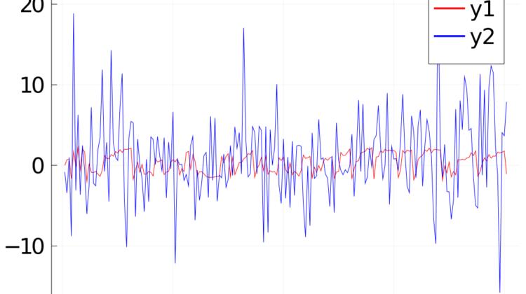
The test result is not good. Here is the plot of the predicted value y1 (red) and the training data y2 (blue). The predicted value cannot fit with the actual value.
You can observe that the actual value is highly fluctuating, that may cause the Gradient Decent cannot converge. Therefore, I try to use moving averge to smoothen the data. I compute the 10-day moving average before the PCA dimension reduction. I apply the 10-day moving average on both input variable sand target variable.
pct = percentchange(ts)
ma = moving(mean, pct, 10)
Here is the plot of the prediction y1 (red) and the training data y2 (blue). The prediction can well fit the actual line. Bingo!
I re-run the training by holding out the last 250 days of data for verification and testing. The result is still good.
Data Leakage?
For fear that the improvement of the result is caused by the data leakage in the moving average computation, I revisit the calculation in details.
The input variables are the values from time i to i+seqlen-1. The moving average is taking the mean of that value with the values of previous 9 days. Therefore, it will not have the future value at time i+seqlen. Although I also take the moving average for the target variable, it still contains the future value at time i+seqlen.
To play safe, I try to run the same model on other target data. If the good result is caused by data leakage instead of the data correlation, I would get the similar result for other target data. I tried the stocks: SQ, GLD, and 2840.HK. SQ is a NASAQ stock related to Bitcoin. GLD and 2840 are the Gold ETF in US market and HK market. Here is the fitting of the training data. The result showed that target data with less correlation cannot fit into the model well.
Comment on Julia
Although Julia is claimed to be fast in computation, it is not easy to use because of the strict typing. Especially the DataFrame is not as handy as Python Pandas DataFrame.
Besides, compilation overhead will make the code slow to run at the first time. It will take some time for pre-compilation when you import the packages with the command “using”.
You can checkout the full code in my git repo.